
During the Winter of 2023, I had the wonderful opportunity to work as a Software Engineering Intern on the SQL Queries team at Cockroach Labs. During the scope of this internship, I found myself working with indexes and specifically implementing forward indexes on columns storing JSONB, which resulted in speeding up query execution time by up to 98% in some cases! This blog post will go over the motivations for the implementation of these indexes, the main challenges that came up with the implementation, and some demonstrations of the staggering results.
What are database indexes?
In the wide world of databases, information stored in tables is required to be retrieved with consistency as well as with high speed. A naive method of locating data within a table lies in scanning each row of the table and processing it, if required. This works well for a query intended to run on a table consisting of a few hundred rows. However, as is the case in many applications that use CockroachDB, this is a problem for tables consisting of a million rows. The same task of scanning each and every row present in such a table proves to be time consuming and inefficient to say the least. How can we do better?
Most databases make use of data structures, called indexes, that are designed to improve the performance of locating data at the expense of additional storage for a given database. This is done by creating copies of columns we want to index our data on wherein these copies also contain a link to the original row of the table since its retrieval could be required. There are different types of indexes and the type of an index is often determined by the structure of data that gets stored in them. Broadly speaking, CockroachDB makes use of forward indexes as well as inverted indexes, both of which will be discussed in upcoming sections.
Phew, so much theory! Let’s make this a little more practical and fun. I intend to demonstrate the power that comes with an index by creating a table, called Manchester, which will consist of the following rows: Player, of type JSONB, and jersey_number, of type Integer, depicting players from Manchester United and the jersey numbers that they don, as of 25th April 2023.
It is also important to note that during the creation of a table in CockroachDB, an implicit column called rowid will be created in the absence of an explicit Primary Key, as in this case. This implicit column is designated as the Primary Key of the table.
RELATED
How to use indexes for better workload performance
Running the following commands should create the table and insert some values:
CREATE TABLE manchester (jersey_number INT, player_info JSONB);

INSERT INTO manchester VALUES 	(25, ’{“Name”: “Sancho”, “Foot”: “Right”}’'),
(21, ‘{“Name”: “Anthony”, “Foot”: “Left”}’'),
(8, ‘{“Name”: “Bruno”, “Foot”: “Right”}’'),
(10, ‘{“Name”: “Rashford”, “Foot”: “Right”}’');


Manchester

|  (Implicit) 	| jersey_number 	| player_info                           	|
|-------------	|---------------	|---------------------------------------	|
| 500         	| 25            	| {“Name”: “Sancho”, “Foot”: “Right”}   	|
| 710         	| 21            	| {“Name”: “Anthony”, “Foot”: “Left”}   	|
| 811         	| 8             	| {“Name”: “Bruno”, “Foot”: “Right”}    	|
| 912         	| 10            	| {“Name”: “Rashford”, “Foot”: “Right”} 	|
Additionally, CockroachDB uses the Pebble Storage Engine to read and write data to the disk. Pebble is a key-value store and requires data from tables, such as the one above, to be stored in a key-value fashion. Thus, data from the above table will get mapped appropriately to be stored in the following fashion (simplified version for an easier understanding):
| Key       	| Value                                     	|
|-----------	|-------------------------------------------	|
| 112/1/500 	| 25, {“Name”: “Sancho”, “Foot”: “Right”}   	|
| 112/1/710 	| 21, {“Name”: “Anthony”, “Foot”: “Left”}   	|
| 112/1/811 	| 8, {“Name”: “Bruno”, “Foot”: “Right”}     	|
| 112/1/912 	| 10, {“Name”: “Rashford”, “Foot”: “Right”} 	|
Hmm. What and how were these two columns developed from our original table? Let’s take a closer look at the very first row to devise a pattern:
• 112/1/500 – This path consists of the table ID of the Manchester table (112), the Primary Index ID (1) and the Primary Key (500) which points to the implicit ID row as mentioned earlier.
• 25, Sancho - This path contains the values taken from the jersey_number and the player_info columns.
Now, let us construct a query with a specific constraint and run it on this table.
SELECT player_info FROM manchester WHERE jersey_number >= 10 AND jersey_number <= 21
The execution engine now has to scan through each row of the table above and process the jersey number to evaluate if it fits our criteria. This shall end up looking as follows:

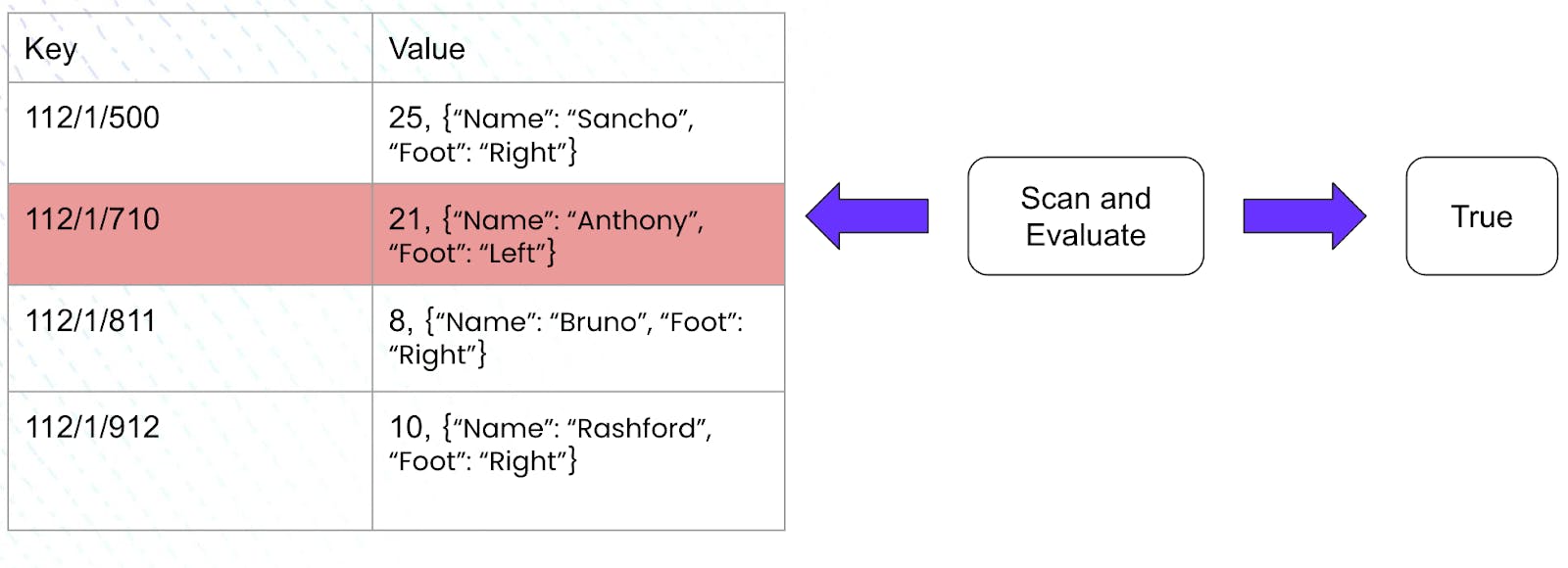
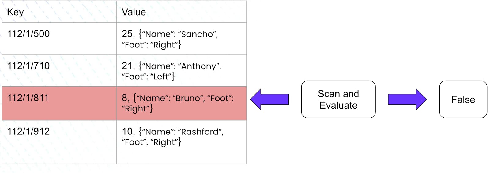

It is imperative to note that in this case, where we did not have an index, the execution engine had to scan every row of the aforementioned table. Since our table consisted of only 4 rows, this did not seem difficult. But what if our table consisted of a million rows? Can we do better than scanning each row and processing it to check if it meets our criteria?
Yes. The creation of an index on the jersey_number column could result in better performance. Creating such an index now results in the creation of a new table consisting, once again, of key-value columns.
RELATED
How to build a payments system that scales to infinity (with examples)
The key columns, in this case, consist of similar paths as the previous example along with the addition of values present in the jersey number column. This is because we shall be creating an index on this specific column. The value column shall contain the values from the player_info column and is done with the help of the STORING keyword.
Let us create an index by running the following command:
CREATE INDEX on manchester (jersey_number) STORING (player_info);
| Key          	| Value                                 	|
|--------------	|---------------------------------------	|
| 112/2/8/811  	| {“Name”: “Bruno”, “Foot”: “Right”}    	|
| 112/2/10/912 	| {“Name”: “Rashford”, “Foot”: “Right”} 	|
| 112/2/21/710 	| {“Name”: “Anthony”, “Foot”: “Left”}   	|
| 112/2/25/500 	| {“Name”: “Sancho”, “Foot”: “Right”}   	|
Upon taking a closer look at the very first row of this newly created index, we observe:
112/2/8/811 – This path consists of the table ID of the Manchester table (112), the Secondary Index ID (2), the value present in jersey_number column (8) along with the primary key (811) associated with this entry in the original table.
{“Name”: “Bruno”, “Foot”: “Right”} - The value, present in the player_info column, corresponding to the jersey_number of 8
It is also imperative to note the resulting table created is sorted on the values that are present in the indexed (jersey_number) column. These values, in this example, are present as the second-last parameter for a given path in the key column.
But does maintaining a specific sorted order help us in any way? Let us take a closer look at the execution engine by running the same query we ran previously:
SELECT player_info FROM manchester WHERE jersey_number >= 10 AND jersey_number <= 21
The execution plan developed in this case is smart in the sense that it now uses a seek operation to state that scanning should commence from the first row where the jersey_number is equal to 10. Since the rows in the index are sorted in nature, the plan realizes that all preceding rows will have values less than 10 and thus do not meet our constraint. Additionally, the execution engine also stops scanning after the last row consisting of a jersey_number less than or equal to 21. Once again, due to the sorted nature of the rows, the plan realizes that all the rows after this one, if any, shall consist of jersey numbers greater than 21 thereby not meeting our constraint. The execution plan conveys this information by generating spans consisting of bounds which help the engine conduct its scan in a better fashion. For this very example, the scans generated would be:
[/10 - /21]
Upon converting the aforementioned abstractness to some visualization, the execution engine works as follows:
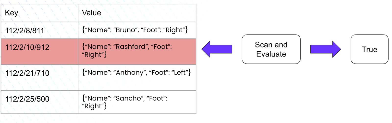

An interesting point to note here is the performance of an index. The creation of an index, in this example, led us to only scan 2 rows out of the 4 in total. On the other hand, running the same query on a table with no index resulted in a full table scan where all 4 rows were evaluated to generate the result.
The execution plans in the two cases compare as follows where the difference is evident.
Execution plans with an Index

Execution plans without an Index

What is JSONB?
Before we talk about having these indexes for JSONB values, I would like to spend some time talking about what JSONB is. Let’s go ahead and address the elephant in the room: What exactly is JSONB?
JSONB is a column type supported by Postgres that allows users to store and manipulate JSON documents directly in their database. It’s distinguished from Postgres’s plain JSON column type in that it stores a binary representation of the documents, rather than the raw JSON string.
In CockroachDB, JSONB currently can be indexed with inverted indexes. These indexes differ from the forward indexes described above as they store each path of a given JSON document in a separate row. This is especially useful when users want to search over a specific subset of data that is found in JSON documents.
Using the same example as above, if we were to create an inverted index on the player_info column:
|  (Implicit) 	| jersey_number 	| player_info                           	|
|-------------	|---------------	|---------------------------------------	|
| 500         	| 25            	| {“Name”: “Sancho”, “Foot”: “Right”}   	|
| 710         	| 21            	| {“Name”: “Anthony”, “Foot”: “Left”}   	|
| 811         	| 8             	| {“Name”: “Bruno”, “Foot”: “Right”}    	|
| 912         	| 10            	| {“Name”: “Rashford”, “Foot”: “Right”} 	|
The original table leads to the following index being created:
| Keycol (jsonpath + primary key) 	|
|---------------------------------	|
| ../Foot:left/710                	|
| ../Foot:right/500               	|
| ../Foot:right/811               	|
| ../Foot:right/912               	|
| ../Name: Anthony/710            	|
| ../Name:Bruno/811               	|
| ../Name:Rashford/912            	|
| ../Name:Sancho/500              	|
|                                 	|
Now, running a query on such an index would result in using the primary keys, present as the last parameter in a path, as references to the rows in the original table which will be used for extracting the desired information:
Select `jersey_number` from manchester where `player_info`->foot = ‘“right”’;

These indexes are held responsible for searching over sub-values that could be contained inside of JSON documents. More information on inverted indexes can be found here.
However, what if a specific user was not interested in a sub-value of a JSON document? What if the component of interest was to search for a very specific JSON document with a very specific structure? This is where forward indexes would come in handy since they have the capability to store the entire value, as seen previously!
Why didn’t CockroachDB have JSONB in forward indexes before?
The main property that comes with a forward index is that it sorts the data that gets indexed. This sorted behavior is also a performance booster, as was seen in the previous sections. Indexing on a given column is thus possible if a lexicographical ordering for the column datatype is present in CockroachDB. In the case of primitive data types such as integers and strings along with data types such as arrays, a lexicographical ordering is defined in CockroachDB, therefore allowing them to be forward indexable.
However, who decides if ‘“a”’::JSONB > ‘[1, 2, 3]’::JSONB? How do we know if two JSON objects consisting of the same key-value pairs in different orders are to be sorted differently? There were many questions left unanswered in this department.
Thus, a strong lexicographical order had to be defined since that would form the basis on which forward indexes could be implemented!
JSONB Semantic Ordering
A JSON value can be one of seven types:
true,
false,
null,
a UTF-8 string,
an arbitrary-precision number,
an array of zero or more JSON values,
or an object consisting of key-value pairs, where the keys are unique strings and the values are JSON values.
The following rules were kept in mind for the semantic ordering of JSON, as defined in the postgres documentation (link):
Object > Array > Boolean > Number > String > Null
Object with n pairs > Object with n-1 pairs
Array with n elements > Array with n - 1 elements
Moreover, arrays with equal number of elements are compared in the order:
element1, element2, element3, ….
Objects with an equal number of key value pairs are compared in the order: key1, value1, key2, value2, ….
CockroachDB currently encodes SQL data into key-value pairs. Moreover, it also converts SQL data types into byte slices, present in these key-value pairs, which are interpreted by Pebble. These encoded fields start with a byte (a tag) which indicates the type of the SQL Datum. For example, the SQL type STRING has a special byte marker in its encoding. More information about how Cockroach encodes data can be found here.
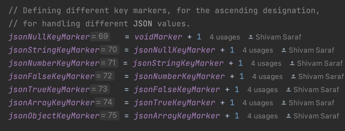
In order to satisfy property 1 at all times, tags were defined in an increasing order of bytes. These tags, for the ascending designation, were defined in a way where the tag representing a JSON object is a large byte representation for a hexadecimal value (such as 0xff) and the subsequent objects have a value 1 less than the previous one, where the ordering is described in point 1 above.
Additionally, tags representing terminators were also defined. There will be two terminators, one for the ascending designation and the other for the descending one, and will be required to denote the end of a key encoding of the following JSON values: Objects, Arrays, Numbers and Strings. JSON Boolean and JSON Null are not required to have the terminator since they do not have variable length encoding due to the presence of a single tag (as explained later in this document).

Keeping these rules in mind, an encoding was devised. This encoding would follow the lexicographical ordering, as described above, which would in turn allow JSONB values to be forward indexable.
JSONB Key Encoding
Since there are 7 different JSON value types, as described in the earlier section, each JSON value type has a unique form of encoding. This section aims to explain the encoding in detail by demonstrating how each JSON value type is encoded:
Null
A JSONB null is stored solely as the tag representing the type.
String
A JSONB String is stored as:
a JSONB String tag
a UTF-8 string
JSONB terminator tag
Number
A JSONB Number is stored as:
a JSONB Number tag
encoding of the number using CRDB’s Decimal encoding.
JSONB terminator tag
Boolean
It is imperative to note that the following query results in “true” in postgres:
select ‘true’::JSONB > ‘false’::JSONB;
Thus, instead of a single Boolean tag (which was described above), two separate tags, one for true and one for false, shall be present. Moreover, the tag for true will have a higher value, in bytes, than the tag for false due to the above query being true.
Thus, a JSONB Boolean is stored as just the tag depicting its type.
Array
A JSONB array is stored as:
a JSONB array tag
number of elements present in the array
encoding of the JSON values
JSONB terminator tag
Object
An interesting property to note about a JSON object, while considering its possible encoding, is the fact that there is no order in which JSON keys are stored inside the object container. This results in the following query to be true (tested inside of psql):
select '{"a": "b", "c":"d"}'::JSONB = '{"c":"d", "a":"b"}'::JSONB;
Thus, it is important to sort the key-value pairs present within a JSON object. In order to achieve a sorting “effect”, encoding will be done in a fashion where all the key-value pairs will be sorted first according to the encodings of the current keys of these pairs. This will be followed by an encoding of each key and value present in these pairs and concatenating them to build the resulting encoding. The key and value encodings, of each such pair, will be intertwined to keep the property that the resultant encoding shall sort the same way as the original object.
Thus, a JSONB object is stored as:
a JSONB object tag
number of key-value pairs present in the object
an encoding of the key-value pairs where the pairs have been sorted first on the encodings of the keys.
JSONB terminator tag
Additionally, having a JSONB semantic ordering and an encoding that now follows this ordering has helped enable the functionality of performing ORDER BY on JSONB columns! Take a peek at the last section for a pleasant surprise!
Forward indexes live in action!
Let us first create a table consisting of an integer and a JSON column. Initially, this table shall not consist of any forward indexes on the JSON column.

Let’s now add 10,000 rows of randomly generated values in this table.

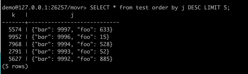
This table now contains data that looks like this:

Now, let us run a query searching for a very specific object present inside this table and note down its statistics.

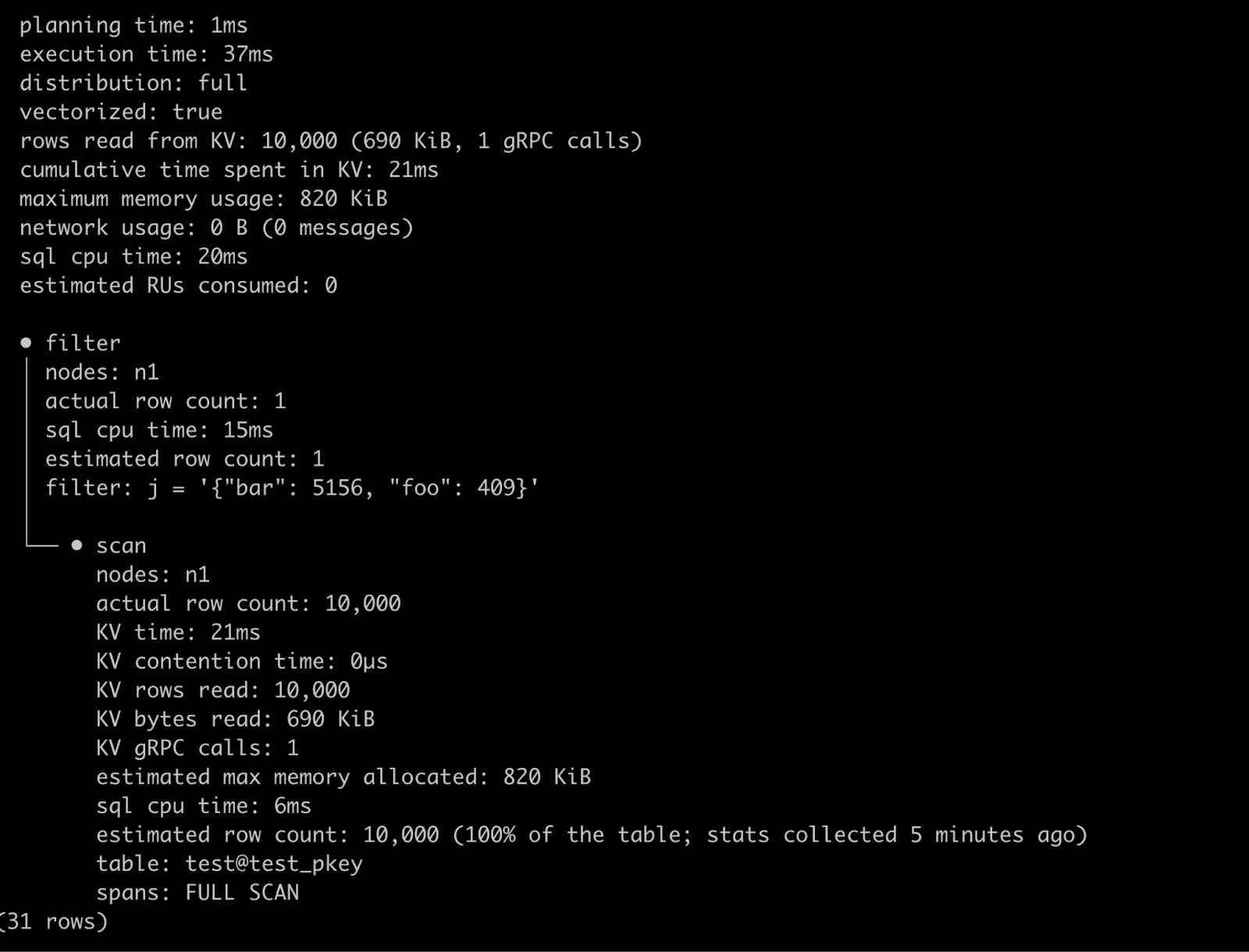
As we can see, the execution engine had to perform a full table scan which searched 10,000 rows until it found the row meeting our constraint. Moreover, the total execution time to generate the result was 37 ms.
Let us now go ahead and create a forward index on the JSON column to compare the statistics generated after running the same query.

Running the same query now produces:

Notice, with the presence of an index, spans are created which has reduced the overall execution time to 2 ms. In this case, the execution engine ended up reading only 1 row of the 10,000 ones present.
In other words, we notice a 94.59% decrease in the execution time of our current query!
Lastly, as promised in the previous section, we can also ORDER BY JSON columns in both ascending and descending designation:

I hope you enjoyed reading about some of the work that I did during my time at Cockroach Labs! During my time at the firm, the Queries team provided me with an ideal platform to devise solutions to problems that have a large scope in today’s world. I will always be grateful for this wonderful opportunity. Lastly, I would like to specifically thank Becca, my manager, Marcus as well as Tommy for their continuous support during my time at Cockroach Labs!