Support for spatial data and spatial indexing is one of the most requested features in the history of CockroachDB. The first issue requesting spatial data in CockroachDB was opened in October 2017, and closed on November 12, 2020 with the release of spatial data storage in CockroachDB 20.2.
Spatial data, sometimes called geospatial data, is data that contains information about geographic (and geometric) features, with PostGIS being one of the most popular spatial data extensions in use. CockroachDB’s spatial data storage and processing features are compatible with PostGIS, while also providing the scale and resilience of CockroachDB.
This blog post discusses how we built spatial indexing in a horizontally scalable, dynamically sharded database. It also covers why simply using PostGIS on top of CockroachDB was not an option, since the R-tree indexing that PostGIS relies on is not compatible with how CockroachDB achieves dynamic horizontal scaling.
Background: Two Common Approaches for Spatial Indexes
Current approaches to spatial indexes fall into two categories. One approach is to “divide the objects”. This works by inserting the objects into a balanced tree whose structure depends on the data being indexed. The other approach is to “divide the space”. This works by creating a decomposition of the space being indexed into buckets of various sizes.
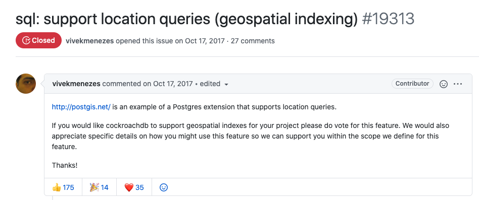
In either approach, when an object/shape is indexed, a “covering” shape(s) (e.g. a bounding box) is constructed that completely encompasses the indexed object. Index queries work by looking for containment/intersection between the covering shape(s) for the query object/shape and the indexed covering shapes. This retrieves false positives but no false negatives. For example, the following diagram shows three shapes A, B, C with the corresponding covering shapes in dotted lines. The coverings of A and B intersect with each other, but don’t intersect with the covering of C. An intersection computed using the index will produce a false positive that A and B intersect, which will be eliminated by exact intersection evaluation over the actual shapes.
Spatial Index Approach #1: Divide the Objects
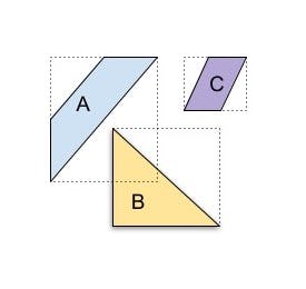
PostGIS is a notable implementation of divide the objects. It maintains an “R tree” (rectangle tree) which is implemented as a Postgres “GiST” index. The covering shape used by PostGIS is a “bounding box” which is the minimal rectangle that encompasses the indexed shape. The following shows an example of an R tree where the red (solid) rectangles show the bounding boxes, and are the leaf nodes in the corresponding tree. The blue (dashed) rectangles are the intermediate nodes, and contain all the bounding boxes in their sub-tree. A search starting from the root can omit sub-trees that have no overlap. For example, consider a search for shapes that intersect with the yellow triangle labeled B, shown with its bounding box. The search at the root will omit R2. Then at the child, it will omit R3, and explore both R4 and R5. When exploring R5, neither R13, R14 are relevant, while in R4, only R11 is relevant.

[Image Credit: Radim Baca and Skinkie from Wikipedia]
Spatial Index Approach #2: Divide the Space
The other approach for spatial indexes is to “divide the space” into a quad-tree (or a set of quad-trees) with a set number of levels and a data-independent shape. Each node in the quad-tree (a “cell”) represents some part of the indexed space and is divided once horizontally and once vertically to produce 4 children in the next level. Each node in the quadtree has a unique numeric ID.
Divide the space algorithms tend to use clever strategies for the unique numeric cell-IDs with important guarantees:
The cell-IDs of all ancestors of a cell are enumerable.
The cell-IDs of all descendants of a cell are a range query.
The cells of nearby cell-IDs are spatially near.
The S2 library from Google is an example of this approach for dividing the earth and assigns cell-IDs using a Hilbert curve.
The following shows points, depicted as small circles, being indexed in a quad-tree, where the squares of various sizes are the quad-tree cells.
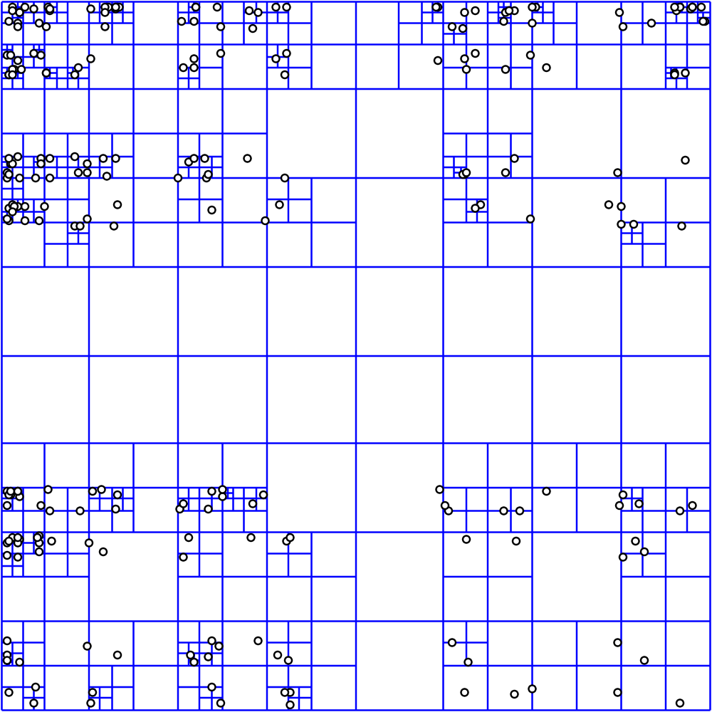
[Image Credit: David Eppstein - self-made; originally for a talk at the 21st ACM Symp. on Computational Geometry, Pisa, June 2005]
When indexing an object, a covering is computed, often using some number of the predefined cells. Ancestors and descendants can be retrieved by using the cell-ID properties above.
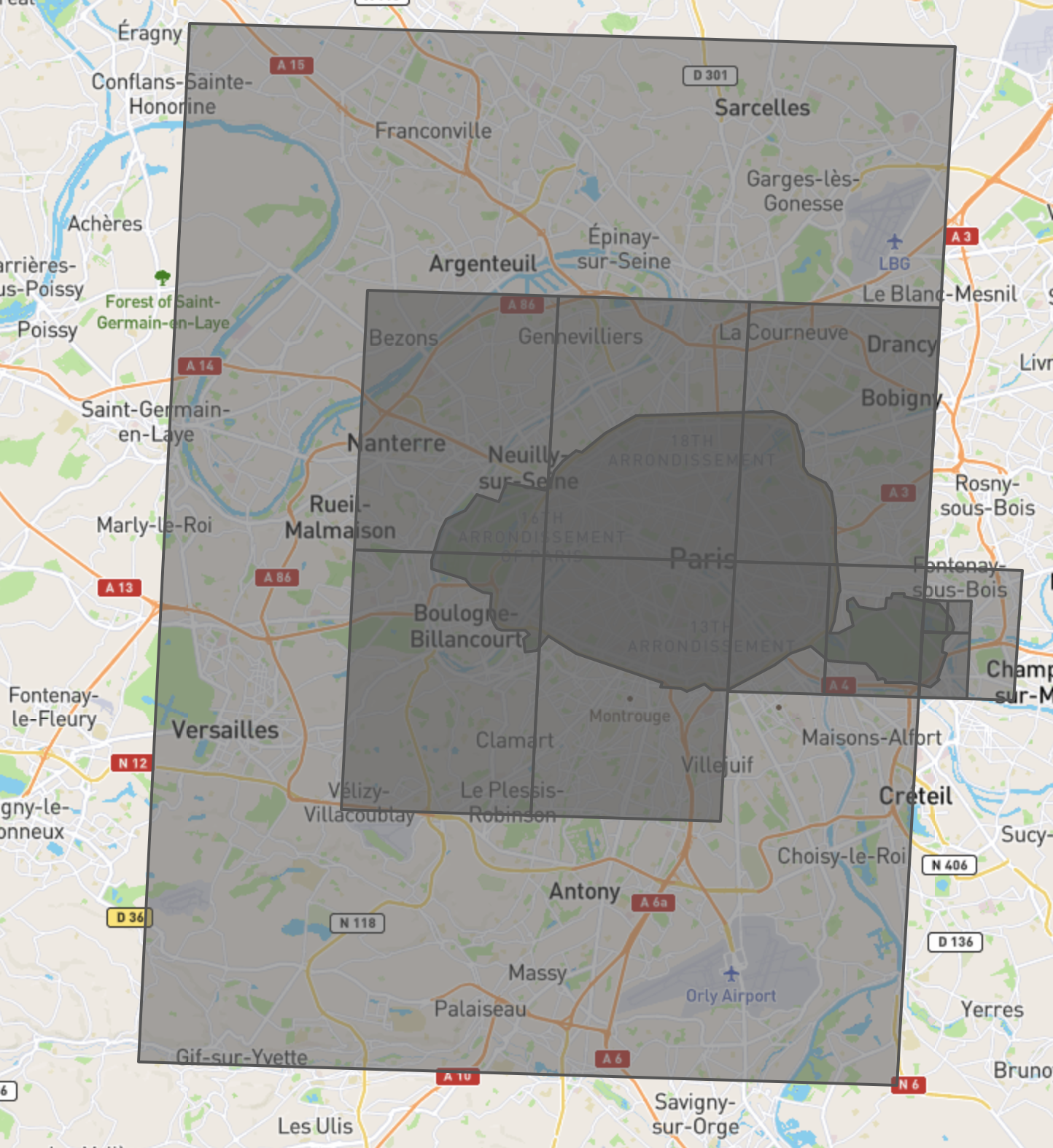
The number of covering cells can vary per indexed object. There is an important tradeoff in the number of cells used to represent an object in the index: fewer cells use less space but create a looser covering. A looser covering retrieves more false positives from the index, which is expensive because the exact answer computation that’s run after the index query is expensive. However, the benefits of retrieving fewer false positives can be outweighed by how long it takes to scan a large index. The following shows both 4 and 8 cell coverings of the city of Paris constructed using the S2 library. Users can construct such a visualization using CockroachDB’s ST_S2Covering function and geojson.io as described here.
Because the space is divided beforehand, it must have finite bounds. This means that Divide the Space works for GEOGRAPHY (spherical/spheroid geometry), and for GEOMETRY (planar geometry) when the part of the plane that will be used is bounded. We discuss later how we configure the bounds for GEOMETRY, and how we handle the case of a shape exceeding the bounds.
Why We chose the “Divide the Space” Approach for CockroachDB
CockroachDB is a dynamically sharded, horizontally scalable SQL database, that arranges all data into a lexicographic total order. As the workload increases, tables and indexes are split into ranges, consistent with this order, and ranges are moved between nodes to balance the load. Ranges can later be merged when the load decreases. The activities relating to range splitting/merging/rebalancing are localized to the affected ranges and do not affect other ranges, which is key to achieving horizontal scaling. A divide the objects approach is incompatible with this scheme since:
The shape of an intermediate node is dependent on many of the indexed shapes, which creates a non-localized dependency.
A general multi-dimensional structure cannot be directly represented in a lexicographic totally ordered space.
For these reasons, CockroachDB uses a divide the space approach, leveraging the S2 library. The totally ordered cell-IDs are easily representable in CockroachDB’s lexicographic total order.
This choice comes with some additional advantages: (a) bulk ingestion becomes simple, and (b) compactions in our log-structured merge tree (LSM tree) approach to organizing storage can proceed in a streaming manner across the input files, which minimizes memory consumption. In contrast, BKD trees, which are a divide the objects approach, also permit a log-structured storage organization, but, to the best of our understanding, compactions need to load all the input files to redivide the objects.
Index Representation and Querying
Spatial data is indexed as an inverted index that contains the cell-ID and the primary key of the table.
In the example below, the primary key is the city name and shows the city from our earlier example indexed using 4 cell-IDs, where the cell-IDs are computed using the S2 library for cell covering and ID assignment.
Note that a particular cell-ID can be used in the covering for multiple table rows, and each table row can have multiple cell-IDs in the covering, that is, it is a many-to-many relationship.
Queries as Expression Evaluation over Sets
Now we come to the most interesting part – how to evaluate queries using such an inverted index.
Consider a query that is trying to compute what indexed shapes contain a given shape, or more generally trying to join two tables based on this containment relationship. For example, if we had two tables with cities and parks and their corresponding geometries, one could do the following to pair each park with the city it is in.
SELECT parks.name, cities.name FROM parks JOIN cities ON ST_Contains(cities.geom, parks.geom)
We can reduce this problem to: given an actual shape g, find the indexed shapes that contain g. In the join case, g will successively take on the value of each geometry on one side of the join.
The following abstract example illustrates how this is evaluated using an index. In this example c[i] is a cell number. Consider g has the cell covering c[213], c[61], c[64] in a quad-tree rooted at c[0]. In the numbering here, the children of cell c[i] are numbered c[4*i+1]…c[4*i+4] (we are not using a Hilbert curve for numbering, for ease of exposition). The following depicts this covering as a tree with the leaf cells being the covering cells. Note that the paths from the leaves to the root are not the same length.
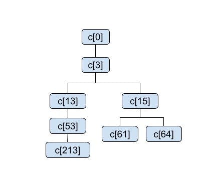
All shapes containing g must have coverings that contain c[213], c[61], and c[64]. Assume a notation index(c), where c is a cell, that returns all the shapes that have an entry in the index for cell c. The indexed shapes that would satisfy the containment function are:
(index(c[213]) ⋃ index(c[53]) ⋃ index(c[13]) ⋃ index(c[3]) ⋃ index(c[0])) ⋂ (index(c61) ⋃ index(c15) ⋃ index(c3) ⋃ index(c0)) ⋂ (index(c64) ⋃ index(c15) ⋃ index(c3) ⋃ index(c0))
One can factor out common subexpressions in the above, which increases efficiency of evaluation. To perform such set expression evaluation, we have developed new distributed query processors, which we discuss in the next section.
New Distributed Query Processors
We introduced two new distributed query processors, inverted filterer and inverted joiner, that apply to the spatial SELECT and JOIN queries. These can evaluate general set expressions derived from the expressions being evaluated. Both these operators can be distributed, for scalable evaluation. The sets are represented as ranges of cells to scan from the inverted index. These processors produce false positives because the coverings are not a precise representation of the original shape. These false positives are subsequently eliminated using a lookup join that retrieves the original shape and does a precise evaluation of the spatial expression. The use of these new processors, and the subsequent lookup join, is automatically planned by our cost-based query optimizer.
The cost-based optimizer uses histograms over the cell-IDs to decide when to use the inverted filterer. The inverted join is currently planned using a heuristic instead of a cost-based approach.
Over 25 of the spatial functions and function variants listed here are accelerated using spatial indexes. Complex expressions which include spatial and non-spatial functions can also be accelerated using spatial indexes.
The following is the EXPLAIN output for our earlier query, which shows both the inverted join and the subsequent lookup join.
> EXPLAIN SELECT parks.name, cities.name
FROM cities JOIN parks
ON ST_Contains(cities.geom, parks.geom);
tree        |         field         |       description
---------------------+-----------------------+--------------------------
                     | distribution          | full
   lookup join       |                       |
   │                 | table                 | parks@primary
   │                 | equality              | (name) = (name)
   │                 | equality cols are key |
   │                 | pred                  | st_contains(geom, geom)
   └── inverted join |                       |
   │                 | table                 | parks@geom_index
   └── scan          |                       |
                     | table                 | cities@primary
                     | spans                 | FULL SCAN
Making queries fast for Real World Data
So far we’ve considered the algorithmic aspects of spatial indexing. The real world data that a spatial database deals with can bring more challenges.
Quality of Cell Covering
Good cell coverings are important for performance. We faced two problems with the quality of cell coverings.
First, polygons with line segments that are near collinear can confuse the covering generator to produce very wide coverings, for example a whole earth covering for the polygon of a city neighborhood. We’ve solved this with a heuristic that recognizes such poor coverings, and falls back to using the bounding box of the shape to generate the covering.
Second, for shapes that are close to a rectangle, cell coverings can be worse than a “divide the objects” index that uses bounding boxes. Our earlier example with Paris is an unusually extreme representation of this problem, where the 4 cell covering is over 5x the area of the original shape. Note that there are also many shapes where a cell covering can be better than a bounding box.
We’ve solved this by developing a scheme that gets us close to the best of both approaches. In our scheme, the inverted index stores both the cell-ID and the bounding box of the original shape. Before using a cell as part of the set expression computation, we use the bounding box to do a fast check of whether the original shape can satisfy the expression, and if not, ignore the key stored with the cell-ID. For certain workloads we’ve observed 3x reduction in false positives with this scheme.
Indexing Bounded Space
We earlier discussed how “divide the space” requires the bounded space to be specified up front. This is not a problem for the spherical/spheroid geometry used for the GEOGRAPHY type. However, this can be a challenge for the GEOMETRY type. We’ve adopted a two-pronged approach to maximize usability and performance for our users:
Ease of Use
When the GEOMETRY column being indexed has a known SRID that corresponds to an earth projection, we automatically infer the finite space for the index. CockroachDB understands over 6000 SRIDs, including all EPSG supported SRIDs.
When the SRID is not known, we use reasonable defaults to reduce the probability of a shape not fitting into the finite space. Finally, if this is not sufficient, the user can specify the bounds when creating the index.
Handling shapes that exceed the finite bounds
We gracefully degrade indexing performance in this case. A shape that exceeds the finite space is clipped and indexed with both the cell-IDs corresponding to the part that falls in the finite space as well as a special overflow cell-ID. The specific geometry being used for the query is similarly handled – if that geometry does not exceed the finite space we do not need to query the overflow cell-ID.
The Spatial Data & Indexing Road Ahead
We plan to continue improving spatial indexing, based on feedback from our users. Examples of areas we are working on are:
Geo-partitioned spatial indexes: A compelling feature of CockroachDB is the support for geo-partitioning, which reduces latency and handles compliance requirements. Inverted indexes, including spatial inverted indexes, currently cannot be geo-partitioned. We are actively working on geo-partitioned inverted indexes.
Left join algorithmic improvements: The plans we generate for left outer/semi/anti joins involving spatial inverted indexes are not as efficient as we desire (unlike inner joins). We are actively working on a new scheme that addresses this problem for “non-covering” indexes. i.e., indexes that cannot fully evaluate the expression, either because they do not contain all the columns needed by the expression, or contain an imprecise column, like the cell covering in a spatial index.
Query improvements for other types with inverted indexes: CockroachDB already supports inverted indexes over JSON and ARRAY types. Queries on these inverted indexes currently do not use the new distributed query processors described above. We are actively working on using these processors for JSON and ARRAY types.
Pebble optimizations for spatial queries: Now that we have an in-house storage engine, Pebble, we have identified and made optimizations to better support inverted index queries, that will be available in the next release.
Don’t hesitate to reach out if you have any feedback on features or capabilities you’d like to see with spatial data. You can post it in the #spatial or #product-feedback channels of the CockroachDB Community Slack.