
Last year the BulkIO team at Cockroach Labs replaced the implementation of our IMPORT bulk-loading feature with a simpler and faster data ingestion pipeline. In most of our tests, it looked like a major improvement: the release notes for CockroachDB v19.2 touted "4x faster" IMPORT. Many a 🎉 reaction was clicked, and the team moved on to new projects. But over the following months, it became clear we had celebrated too soon: we started to get reports of some IMPORTs that, instead of being faster, were much slower or even getting stuck. Armed with a test that could reproduce such a case, we started to dig.
What followed was a search to find out what had happened. We spent weeks digging through the code, reading logs, and running experiments, and building new debugging tools. When we finally figured out what was going wrong, we realized fixing it would require changes at the very lowest layers of our storage system. In the end, the solution hinged upon our recent switch from RocksDB as our key-value store to Pebble, where we were able to add a new algorithmic approach to organizing files that led to a massive improvement, measured at an 80+% reduction in ingestion time time on the standard TPC-C benchmark dataset.
Note: a firm understanding of how RocksDB or other LSM-based storage engines operate will be required for much of this to make sense. For those that want to pause here and brush up on the subject, this is a great introduction to LSM trees.
In this post, we want to walk through our initial rewrite of IMPORT, how we isolated the cause of the slow-downs and, most importantly, how we fixed it. But to start, let's cover some basics.
What Is IMPORT in CockroachDB?
We built IMPORT to make it easier and faster to get large amounts of data into CockroachDB. CockroachDB's SQL layer is built on top of a distributed transactional key-value store. When a row is written via SQL in a normal INSERT statement, the SQL layer encodes the row as bytes. The encoded columns in the table's primary key become the key in that key-value pair and the rest of the columns are encoded in the value. For each row written the SQL layer sends those KVs in transactional Put-requests to the KV layer.
The IMPORT process starts by running the format-specific input reader, like a CSV reader or Avro codec, to extract logical rows from the input data. It then uses the schema to encode those rows into the same byte KV pairs the SQL layer would produce if those rows were sent as INSERTs. But instead of sending the KVs as individual transactional Puts, IMPORT instead assembles them into large SSTable ("SST") files. SSTs are the native storage format used by CockroachDB's on-disk storage engine, so IMPORT can send them to the storage layer to be directly ingested, with minimal per-key processing compared to a Put'ing each key. When sending these files, we take every possible shortcut through various layers of the stack, skipping nearly the entirety of the transaction layer and using clever tricks to avoid making copies when doing things like replicating in the Raft log or writing to the write-ahead log. The result is a process that can bulk-load orders of magnitude faster than running regular INSERTs.
Two-Pass IMPORT
When we first built IMPORT, we used a two-pass approach. Since CockroachDB is a distributed system, we want to distribute the data we're importing across the cluster. For example, if you were importing a file of rows whose keys were uniformly distributed between 1 and 100 into three nodes, you might want to say keys 1 through 33 to go to node 1, keys 34 through 66 to node 2, etc. But when we start an IMPORT of an arbitrary file, we have no idea what the distribution of the keys it will produce is, and thus have no way to specify such a partitioning.
This is what motivated the two-pass approach: we ask every node to read its assigned input files and convert them to KVs twice. In the first pass, they are told to discard all but a small sample of the resulting KVs, which then establishes the distribution of the KVs and partitions them roughly evenly. All of the readers then read and convert their assigned input a second time, this time using that partitioning to route streams of the produced KVs to destination nodes, which can assemble them into SSTables to ingest. One complication though is that SSTables are sorted but the incoming KVs could be in any order depending on the input, so at the destination node, we buffer all the produced KVs to a temporary RocksDB instance on disk until the input is fully read before reading the now sorted buffer back to produce SSTables and send those to be added to the storage layer.
This is how IMPORT worked from its introduction until v19.2. While it was much faster for bulk-loading than running SQL INSERTs, we thought we could do better.
One-Pass IMPORT
In the two-pass IMPORT, we were writing every produced KV to a buffer on disk before reading it back to produce SSTs. But if our goal is to write all the keys to disk, why do it all to the buffer just to then read it back and do it again? Could we just write it directly to our storage instead? And, as long as we were getting rid of the extra write-pass, could we eliminate the extra read-pass too? Unlike the statically partitioned temporary buffers, our actual KV storage layer automatically and dynamically determines when a given node is over-full and splits some of its key range off to rebalance to another node. If we just directly sent out-of-order data, as it was produced, to the KV layer it should spread it around on its own, right?
And thus we set about switching to "direct" IMPORT. In this implementation, we would only do one pass, in which the keys emitted from the frontend would be buffered in each reader but only up to some memory-based limit, then locally sorted and batched into SSTables that could be sent directly to the KV storage layer. This approach cut out the distributed shuffle and sort phase we had been doing prior to adding to storage. Instead, when the readers finished their first read pass and had flushed their buffers, the IMPORT was done. This approach cut out two of three read passes -- the sampling read of the input and reading the buffer -- and one of two write passes -- writing to the buffer -- so it had to be faster, right?
Of course we knew it wasn't quite that simple. LSMs like RocksDB store data in order. Adding data to RocksDB out of order would mean it would need to do more work to get it in-order. But we were already adding out-of-order to our temporary RocksDB, we reasoned, so it couldn't be worse to just do the same to the real one instead. Plus, in many cases the data is dumped by its source system in-order, making buffering to sort entirely wasted work.
Armed with this reasoning, we forged ahead with "direct" IMPORT, and our early benchmarks seemed to show what we expected -- eliminating the sampling phase and the extra write pass made most of our IMPORTs 4x faster. Giving a feature a big speed boost while deleting most of its code seemed like a win/win, and we celebrated shipping it in our v19.2 release.
Examining IMPORT Slowdowns with LSM Tree Visualizations
After v19.2 was released, most feedback on IMPORT was positive -- but we also got reports that some IMPORTs were slowing to a crawl or "getting stuck". We soon realized it was mostly in larger tables that needed to ingest large volumes of out-of-order KVs. This could be when the rows themselves were out-of-order relative to their KV encoding, or was more commonly seen with tables that included secondary indexes. Indexes almost always produce out-of-order KVs. If you consider a "user" table, while user ID 1 and user ID 2 may appear in-order, ID1 might have email xyz@example.com and ID2 might have abc@example.com, so an index on that email column would be in a completely different order than the source rows.
In every case we looked at, we saw that the IMPORT process was blocked sending an SSTable to the storage layer. When we inspected those requests, we found they were being intentionally delayed by a backpressure system built to protect the storage engine and ensure its background maintenance work kept up with incoming data.
The signals that were causing us to delay were either that we had too many files in the least-sorted part of the LSM (L0) or that we had too many bytes that required compaction. Our unsorted ingest had a known edge-case where it could produce many "small" SSTs: if a given reader read a fixed-size buffer of rows that were uniformly distributed over the key-range of a massive table that had been split into many ranges to spread it around a cluster, the subset of that buffer that would be assigned to the SST sent to any one range could be very small. Throwing thousands of tiny files at the LSM is actually much worse for bulk-loading than the old individual Puts we use for normal writes. This is because LSMs have a built-in mechanism for batching up lots of puts into a single file: the memtable. Thus the first optimization we added was a heuristic to fall-back to Puts to the memtable when ingesting an SST that was "too small" to be worth adding to the LSM as a separate file, i.e. where the overhead of a file to compact would outweigh the write-amplification of adding to the memtable and WAL (write-ahead log) and then flushing.
This helped alleviate the cases where the number of files grew too large due to the "tiny SST after sorting problem", but we still saw IMPORTs that, after starting off fast, would suddenly slow to crawl. We noticed that this was usually happening when, for inexplicable reasons, the storage engine compactions would suddenly no longer keep up with the ingestion load and the backpressure would kick in. Why was compaction falling behind so suddenly and why didn't it recover once the backpressure gave it some time to do so? We were stumped at this point, and brought in the help of our colleagues on our storage engine team so we could stare at our logs and metrics together.
The "Inverted" LSM Tree
One thing common to all the cases where the IMPORT slowed to a halt was that the node triggering the backpressure had an "inverted" LSM tree.
Typically, an LSM wants the majority of its data in its "lowest" levels. As new data comes in, if a file contains data that overlaps with an existing file, it has to be placed "above" that other file and then the compactor has to do some work to combine it and move it down. In RocksDB, levels are numbered 0-6, with L0 being the highest/newest, and L6 being the lowest/oldest. The highest, non-L0, non-empty level is called LBase, and typically the LSM has files in L0 as well as LBase - L6. If too much data piles up in an upper-level while you keep adding more data, that additional data will continue to pile up above that level, and you may end up with a top-heavy "inverted" LSM, where new data that might have ingested to a lower level in a well-shaped LSM just keeping piling up at the top, making the problem worse.
This is why those back-pressure systems were added in the first place: to give the compactor a chance to resolve such a situation before it got worse. But in our case they clearly were not working: around the time of the inversion we often saw RocksDB embark on a giant compaction from L0 to LBase which could take it minutes, sometimes ten or more, to complete. During that time, it cannot start other compactions from L0, so once the limit is reached, to prevent the problem getting any worse, the backpressure would kick in and bring the entire job to a standstill.
But we still didn't understand why it suddenly got so bad. What caused this sudden giant compaction? It was clear the out-of-order ingestion was adding lots of overlapping SSTs and that that put more load on the compactor. But we were writing everything out-of-order to the temporary buffer RocksDB before and it never had this problem. Something didn't add up but we were struggling to see what it was.
LSM Tree Visualization
Our co-founder and resident RocksDB expert started work on a small LSM tree visualizer tool that could process the RocksDB manifest and produce a visual timeline of the files and how they overlapped. The visualizer tool though made it much more obvious, as we scrolled through the timeline of one these tests, that right before one of these giant compactions started, we saw an unusual file added to L0. Specifically, it was a very small, in total size file but it was exceptionally "wide" in terms of the key-span it overlapped.
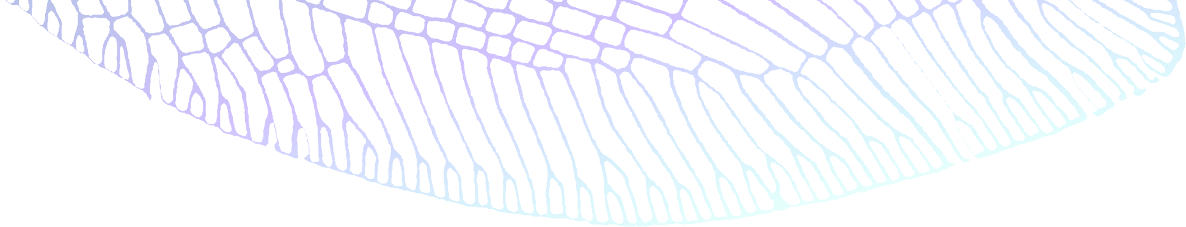
Why is that an issue? Consider the example LSM tree below, where each horizontal line is an SSTable occupying a part of the keyspace:

Figure 1: A simple example of an LSM tree with two levels, and with SSTables visualized as horizontal lines occupying a slice of the keyspace.
For simplicity of explanation, we have defined LBase as L6, so the only non-empty levels of the tree are L0 and L6.
Here, L6 has 4 non-overlapping sstables; all levels outside of L0 are required to not have any overlapping SSTables within themselves. L0 also has 4 sstables, with some overlap between them as well as with L6.
Consider a “flush” happens from memory to L0, adding the red SSTable below:
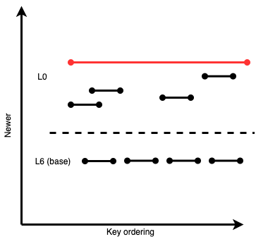
Figure 2: Same LSM example as above, now with a newly added SSTable to L0 that occupies a wide slice of the keyspace, overlapping with all the older files
The wide SSTable itself doesn’t need to be very large in disk size (in our observations, we saw very wide SStables that were only a couple kilobytes large). But it overlaps with all the other files in L0 and L6. If we wanted to move it “out” of L0 and into Lbase, we’d have to run a compaction including all those files (to maintain LSM tree invariants). Many of those overlapping files pulled in from L0 and L6 could be large. Even if the overlapping files weren’t large, the mere presence of these wide files would block other incoming SSTables in that wide key range from being ingested at lower levels, resulting in more and more bytes accumulating above them. There’s a high likelihood that we’d eventually have to do a mega-compaction that would take a while and use up valuable disk bandwidth. All the overlapping files in L6 would have to be rewritten.
If that mega-compaction with the very wide SSTable gets started, while more L0 SSTables continue getting added to the LSM, the LSM would end up looking like this:
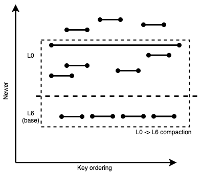
Figure 3: A compaction chosen to compact away the wide L0 file, that ends up picking all overlapping older files in L0 and L6.
The newly added L0 files at the top cannot be added to a running compaction (it’s already running), and they cannot be compacted into L6 as they conflict with older, overlapping, already-compacting files. So at this stage, RocksDB would schedule an intra-L0 compaction to join those files into one L0 file:
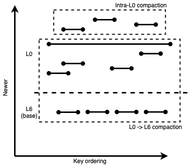
Figure 4: A concurrent intra-L0 compaction being chosen while the mega L0 -> L6 compaction is running
Assuming the smaller intra-L0 compaction finishes before the mega L0->L6 compaction, the LSM would look like this, with the newly-produced file in red:
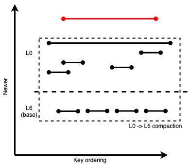
Figure 5: The intra-L0 compaction finished and produced another wide L0 SSTable
We can see how this intra-L0 compaction was a highly unproductive exercise; it ended up producing another wide SSTable out of what were originally narrow ones. This new wide SSTable will continue to require expensive large L0 -> LBase compactions that rewrite most of LBase, and will block any newer files from easily getting compacted out of L0 too.
This begs the question: why were wide SSTables being generated to begin with, especially if they didn’t have many bytes in them? And again, why was this only a problem in directly ingested IMPORTs and not in the previous version, ingesting the same keys?
Sharing a (Key)space Can Be Challenging
Once our visualizer tool made the problematic "wide" file easy to spot, we examined its key bounds and had a breakthrough: its span was the upper-bound of our total addressable logical keyspace, aka "KeyMax". Of course that would overlap with many other files: it overlaps every possible key above its start key! But why did we end up with that as the upper-bound for an SST? Obviously our CSV can't produce a row with that key, as its keys would all be within its assigned table span prefix. This was our first indication that it wasn't just our CSV's produced keys we needed to think about. A little digging revealed that that key was being produced by an unrelated write being done by one of our KV layer's internal housekeeping routines, not our IMPORT. Finally we understood what was different from the old two-pass IMPORT: two-pass IMPORT did its sorting in its own temporary rocksdb, and where the KV's housekeeping writes didn't get mixed into the same files. We finally had our smoking gun. And happily it looked like a quick fix to alter the KV routine to use a more narrowly scoped upper-bound key. We thought we were as good as done.
We excitedly merged the change to the KV's housekeeping routine and re-ran our tests... only to observe the same compaction death spiral. But we had fixed it, hadn't we? Going back to the LSM visualizer, it immediately highlighted another "wide" SST being added and triggering the giant compaction of death. Looking at this file's key-span bounds again revealed that it was IMPORT mixing its data keys with the system's internal keys that was to blame. This time it was internal keys used to store metadata, which are kept under a prefix that sorts at the minimum end of the keyspace, below all table data. When we send a write to a range, the range writes the associated key to its storage but also updates its own internal range metadata for things like number of keys, their size, etc. The range periodically writes its metadata to its metadata key and if both the metadata write and the data write are sent to RocksDB and end up in its memtable together, when that memtable flushes to a file, that file's span will be at least from that metadata key all the way up to that data key, which means it overlaps all other data keys up to the written key. The visualizer made this very apparent: it showed a tiny file appear in L0 overlapped nearly the entire keyspace, and thus immediately triggered our giant compaction of death. Unlike the previous case of KeyMax however, there was no easy way to avoid the writes to the metadata keys this time.
Those familiar with RocksDB might immediately suggest using its "Column Family" feature which provides nearly entirely separate LSMs for logically separate key-spaces. If we stored our metadata keys and table-data keys in separate column families, we'd be all set, right? However changing to do so now would pose a very tricky migration challenge. Alternatively, a less drastic separation could be provided by a feature that manually partitioned one key-space in place, such as has been explored in academic projects like PebblesDB's "guards".
While manual partitioning approaches like those could address our metadata vs table-key spans, the same issue would arise even in a pure table data setting: Our input CSV could have rows in any order, including an order of rows that could generate a similarly "wide" span, e.g. if it had row 0 followed by row 1,000,000,000.
Introducing a New KV-Store: Pebble
During this time, we were building a new storage engine in-house to replace RocksDB. It’s called Pebble (no relation to the above-mentioned PebblesDB), and has been in development since late 2018. Pebble is designed to be compatible with RocksDB in its on-disk format, making bidirectional migrations very straightforward. Written in Go, it’s designed to efficiently implement just the select set of RocksDB features that CockroachDB relies heavily on. We discuss Pebble in this blog post, and it is already the default storage engine for CockroachDB v20.2.
Owning our own storage engine lets us incorporate CockroachDB-specific features and improvements down in the storage engine itself. As part of our import speedup efforts, we reorganized L0 of the LSM into dynamic “sublevels”, where each sublevel can be seen as yet another non-L0 level of the LSM. These sublevels would be ordered by key age, such that keys in newer sublevels will always shadow keys in older sublevels, just like with regular levels. And each sublevel would also contain a set of non-overlapping SSTables, just like other levels. The sublevel organization is a function only of the key age and key span of files, so it is backwards compatible with RocksDB.
How does the switch from RocksDB to Pebble affect our slowdown issue? For one, instead of having to read and merge every L0 file independently for every read and compaction, we can reduce the effort down to only the number of sublevels that are being read; only one sstable would need to be read in every sublevel at a time. Our read amplification gets significantly reduced.
Going back to our earlier example, where L0 files are ordered by age only:
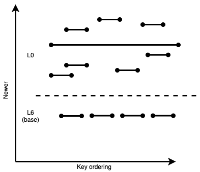
Figure 6: Example from above, with many L0 SSTables, some wide and some narrow.
Here, we have 8 SSTables in L0. Not all of them overlap with all the other files; so reading and merging 8 files every time we do a key read or compaction in L0 is very inefficient. However, if we move files into sublevels while still ensuring that newer keys always remain “above” older keys, the LSM tree ends up looking like this:

Figure 7: Same example, but with L0 organized into sublevels based on key overlaps and file age.
By organizing L0 into dynamic sublevels while still respecting all existing LSM invariants, we’ve managed to reduce read amplification in our example down from 8 to 4. This is already a significant enough improvement. But the extra-wide SSTable in L0.2 is still preventing us from optimizing this further.
Organizing SSTables this way has another benefit: it allows us to easily calculate overlaps across sublevels, as files in each sublevel are sorted by key ordering. Previously, all files in L0 were just sorted by age, making overlaps harder to identify. Once these overlaps are known, we can calculate “split points” to reduce excessive overlapping even further. Any future flushed SSTables would be split at these split points to prevent excessively wide SSTables. In our example, our algorithm would split the L0.2 SSTable into three SSTables:
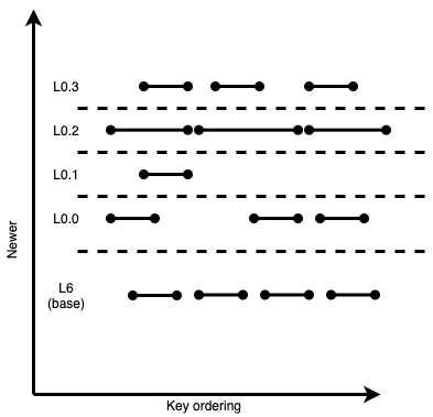
Figure 8: Same sublevel example, but with wide L0 files split at calculated flush points
This can be more efficiently organized as:
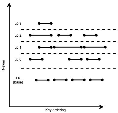
Figure 9: Same example, after “moving down” non-overlapping fragments
The right half of the LSM is only 3 sublevels tall now! A nice improvement, but nothing too groundbreaking. However, when choosing compactions, this gives us three main benefits:
Increased L0 -> LBase compaction concurrency: As there are no super-wide files overlapping all other files, we can schedule more concurrent L0 -> LBase compactions, each of which can operate on a subset of the keyspace without having to rewrite all of LBase or read most files in L0.
Reduced need for intra-L0 compactions: Due to increased concurrency of L0 -> LBase compactions, and because read amplification is now equal to the number of sublevels (and not number of L0 files), there is a significantly reduced need to run intra-L0 compactions.
More efficient compaction picking: The sublevel structure itself tells us all the information we need to know to pick efficient compactions. We know that our goal should be to reduce read amplification in L0 to allow for more writes into it in the future; so we can pick the files that cause the “tallest” peak in the sublevel structure, and prioritize that first.
For our running example, these would be the 3 L0 -> LBase compactions we can pick with compaction #1 being of the highest priority as it would reduce the sublevel height by 1:
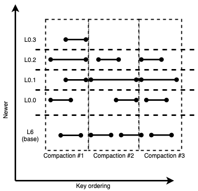
Figure 10: Lack of wide files allows for shorter, more concurrent L0 -> LBase compactions
Since compaction #2 and compaction #3 conflict on one LBase file, both of them cannot be scheduled concurrently. However each of compaction #2, #3 does not need to include more than 3 files from L0. This is critical in reducing the size of compactions. Smaller compactions can result in a healthier LSM because they don’t block other compactions for long durations. And compaction #1 can run independently of the others, concurrently. So in this example two compactions can concurrently run from L0 to L6. This is an improvement over RocksDB, which is limited to running one compaction at a time out of L0.
Additionally, if needed, compaction #1 and compaction #2 can proceed concurrently with an intra-L0 compaction, as shown in the following diagram:
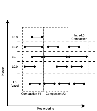
Figure 11: Intra-L0 compactions are also unlikely to produce wide L0 files
Since such intra-L0 compactions are sub-level aware, they do not result in wide files, and therefore maintain sub-level health. In practice, with sublevel-based compactions and flush splits, we see that throughput to move bytes out of L0 is high enough to mitigate the need for intra-L0 compactions altogether. This keeps the write path as fast as possible.
Algorithmic aspects of sub-level compactions
Sub-level compactions are algorithmically more complex than regular compactions for the following reasons:
A compaction can span multiple sub-levels (not just 2 levels like normal compactions).
For backwards compatibility, the sub-level assignment of a file is not stored and is purely a function of the age of data in the file and the key span of that file. This also means that the sub-level assignment for files needs to be (efficiently) recalculated as other files are added and removed from L0.
Consider the sub-levels and files in the following diagram, where the file numbering corresponds to the age of the data (higher number is younger data).
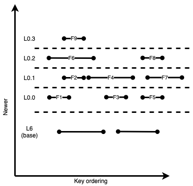
Figure 12: An LSM example with 9 files in L0 of varying widths
As expected, for files that overlap, as we go to higher sublevels the numbering increases. However, it is legal for file F3 to be in a lower sublevel than F2. Since F1 is part of the key span that has a depth of 4, it can be a preferred file to build a compaction candidate. To build the input files for this compaction, one walks up the sublevels looking for overlapping files. This is to reduce future write amplification since compacting only F1 down to L6 means that that data will get rewritten when later compacting F2, F6, F9. Say we include file F2 and then F6. Since F6 overlaps with F4, we need to include F4 and then transitively include F3. Not doing so will violate the LSM invariant by moving younger data for a key to L6 while leaving older data behind in L0. The set {F1, F2, F6, F4, F3} is a valid compaction candidate and this compaction will include the two files depicted in L6. If the total bytes in this candidate compaction are not above a large compaction threshold, we may also include F9 since it reduces write amplification in the future. After the compaction, that included files {F1, F2, F6, F4, F3} from L0, finishes, the LSM would look like the following (assuming no more data was added while the compaction was running).

Figure 13: Same LSM example, after compacting files F1, F2, F3, F4, F6 to LBase
Note that file F9 has moved from sublevel 3 to sublevel 0, because there are no older files overlapping its key space. And sublevel 3 no longer exists, since there are no files that need to be in that sublevel.
The Result: 80% Time Reduction in TPC-C Bulk Import
We have illustrated the sub-level approach using toy examples. Here we show a snapshot of the LSM visualization of a real LSM in the middle of a heavy import. Note that the LSM looks inverted in terms of L0 bytes being very large. This will slowly clear itself when there is spare write bandwidth after the import finishes. But this LSM is healthy in that the read and write amplification have not increased much. Instead of wasting write bandwidth on intra-L0 compactions that produce wide files and leave data in L0, the compactions seen in this import were all moving data from a higher level to a lower level.

Figure 14: Real-world LSM visualization, before sublevels. Note the high count of sstables in L0 (847).
Here’s the exact same LSM revision, except with L0 broken down into sublevels:

Figure 15: Same example, but with sublevels enabled. The same 847 L0 SSTables can be organized into just 13 sublevels.
There are 13 non-empty sublevels in the above example, so the contribution of L0 towards read amplification at this point is 13. Without the sublevels work, L0 would have contributed 847 to read amplification, as that’s the count of all files in L0. This shows how much of an improvement sublevels are, even in situations where the LSM is temporarily in a less-than-ideal shape.
Our real-world-like import example consisted of about 5TB of data to import, using the stock table in our TPC-C workload generator, with warehouse count set to 50,000. Before making any of the improvements outlined in this blog post, a CockroachDB cluster running on 10 c5d.4xlarge nodes on AWS on ephemeral SSDs would take 6.5-10h for the import job to finish, after which it would be another 3-6h for compaction activity to quieten down.
After making the above improvements, we were able to bring it down to a much more reliable 1h15m-1h30m for the import job, and an additional 30 mins for compactions and range merge activity. That’s a time reduction of more than 80%!
Conclusion
This project started with a change at one layer of the system that had unexpected and unintended effects on another. This led us on a journey of spelunking into the lowest layers of CockroachDB, RocksDB and eventually Pebble. It was frustrating at times and hit some dead-ends along the way, but ultimately proved fruitful. We came away with not only a faster IMPORT but also a storage layer better equipped to better handle more varied write distributions, which could occur in other workloads as well. We’re excited to make the IMPORT process a better experience for our users, and will continue to do so in future releases of CockroachDB.
And if visualizing LSM trees is your cup of tea, we’ve got good news: Cockroach Labs is hiring.