

Achieving low latency reads in a transactionally consistent, multi-region database is a unique challenge. In CockroachDB, two approaches are frequently used: geo-partitioning data so that it is located in the region where it is accessed most frequently, and historical reads, which read slightly stale data from local replicas. However, there is a third approach that is used less frequently because it fits a narrower use case: global tables. Global tables offer low-latency non-stale reads from all regions at the cost of higher write latency, and they can be used in many cases where the workload has a high read to write ratio.
One of the challenges with global tables is high write latency, which can be as high as 800ms with the default cluster configuration (as of 22.1) in a cluster spanning the globe. This article explores techniques for optimizing write latency of global tables, which can be used to lower the latency to 250ms or less. Although global tables are not appropriate for all use cases, optimizing write latency can eliminate a barrier to adoption for workloads with a high read to write ratio.
A peek under the hood
Tables in CockroachDB can be marked as global tables by a simple declarative SQL statement or a change to the table’s zone configuration. When a table is marked as a global table, transactions to the table’s ranges use the “non-blocking transaction” protocol, a variant of the standard read-write transaction protocol. The term “non-blocking” comes from the fact that, outside of failure scenarios, reads don’t block on the atomic commit protocol of writes. This is because writes to these ranges are created slightly in the future, making them invisible to current time reads. To ensure that followers have successfully replicated changes, write transactions incur a high wait time, during which time replication to followers is ensured.
To understand how global tables work, let’s consider two types of timestamps: transaction timestamps and closed timestamps.
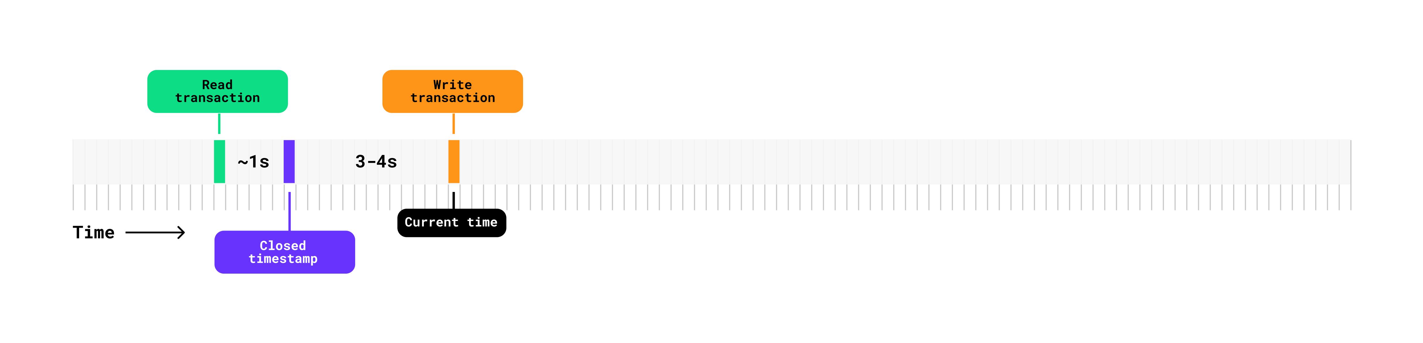
When a transaction is created in CockroachDB, it is assigned a timestamp. In typical transactions, the timestamp corresponds to the node’s current time, determined by its hybrid logical clock (HLC). However, when a transaction writes to a global table, a timestamp is chosen that is slightly in the future, typically hundreds of milliseconds, essentially scheduling it for the future time. After the transaction commits, control is not returned to the client until the current time catches up to the future write timestamp. This wait time is why global tables have higher write latency. It is sometimes referred to as the “lead time for global reads”.
While transaction timestamps correspond to individual transactions, closed timestamps correspond to entire ranges. A closed timestamp is a time below which (i.e., earlier than) no new data will be written, and is determined by the range’s leaseholder. The closed timestamp is propagated from the range’s leaseholder to its followers either via the raft log, when a write occurs, or via a side transport mechanism at regular intervals.
Typical ranges set the closed timestamp several seconds in the past. This allows followers to serve exact and bounded staleness reads at a time ~4 seconds in the past.
Write transactions have timestamps at current time and the closed timestamp is emitted several seconds in the past. This makes it possible for a consistent stale read at an earlier time where it is guaranteed that no new writes will occur.
However, global table ranges set the closed timestamp slightly in the future. This enables reads at current time on followers, since data in the interval between the current time and the in-the-future closed timestamp is immutable. Followers will never see new writes during this interval.

Write transactions have a timestamp in the future. The closed timestamp is propagated to follower along with the write. It is guaranteed that no new writes will occur below the closed timestamp. The lead time for sender ensures that the write is fully propagated to followers. Strongly consistent, non-stale reads can occur at current time on any follower.
Read latency in global tables can be as low as several milliseconds, similar to stale follower reads; however, there is one situation where the read latency can be significantly higher. This occurs when a future write passes into a conflicting read’s uncertainty window defined by the node’s maximum clock offset. During this interval, causality cannot be strictly determined, so the read must wait until the future transaction becomes present time.

When the timestamp for a write transaction in a global table is within the uncertainty window, a read to any data impacted by that write will need to wait until the uncertainty window passes, incurring higher read latency. This is because during the uncertainty window it is not possible to determine the ordering of the two transactions.
Because unexpectedly high read latency can occur when a write enters a read’s uncertainty window defined by the maximum clock offset, global tables are recommended for use cases, such as reference or lookup tables, that have a high read to write ratio. In addition, writes should be distributed across a wide range of rows or occur infrequently, and write transactions should not be held open for extended periods, which increases the likelihood of passing into the uncertainty interval.
More than just reference tables
Although global tables are often recommended for rarely changing reference tables, such as a zip code database, they can be used effectively in situations where a workload has a high read to write ratio and high write latency can be tolerated.
In general, the following characteristics are a good starting point for evaluating whether a table is a good candidate for global tables:
Reads and writes are well distributed throughout the table
Higher write latency can be tolerated (250-800ms, depending on configuration)
Low read latency (i.e., region local, < 10ms) is needed
As an example, consider a table that stores metadata for a company’s critical infrastructure. The infrastructure has hundreds of thousands of components but each is updated infrequently. As a whole, the table sees dozens of writes per second well-distributed across the table’s rows. However, the company has hundreds of services across multiple global regions that need low latency, non-stale access to the infrastructure data. Reads are on the order of hundreds of thousands per second. Though not a “reference” table, this table would be a prime candidate for a global table.
Calculating write latency
In typical CockroachDB tables, write latency is largely determined by the time required to achieve quorum via the raft consensus protocol. This is a factor of the network latency between the voting replicas. In global tables, however, write latency is determined by how far into the future the transaction is written. With global tables, this is referred to as the “lead time at sender” or the “lead time for global reads”. Quorum is still required for writes to global tables, but it occurs concurrently during this lead time and is always shorter than the overall lead time.
Lead time, which is our proxy for write latency, is determined by the sum of 3 components: maximum clock offset, a fixed buffer time and the maximum closed timestamp propagation time.
lead time at sender (aka write latency) =

  [max clock offset] + [buffer time] + [maximum propagation time]
Maximum clock offset is defined at node startup and defaults to 500ms, as of v22.1. Buffer time is a fixed constant of 25ms, which is designed to smooth out network blips or anything that could affect propagation of the closed timestamp. Because the closed timestamp has two propagation paths, via the raft log or via a side transport mechanism, the maximum propagation time is determined by taking the maximum of these two separate calculations.
maximum propagation time =

  max(raft propagation time, side transport propagation time)
Raft propagation time is calculated by the following equation that takes into account the maximum network round-trip time and a fixed raft transport overhead.
raft propagation time =

  [max network rtt] * 3/2 + [raft transport overhead]
By default, a maximum network round-trip time of 150ms and the raft transport overhead is a constant defined as 20ms.
The time required for side transport propagation is as follows:
side transport propagation time =

     [max network rtt]/2 + [side transport interval]
The default maximum network round-trip time of 150ms applies here, as well, and a side transport interval of 200ms is used. The side transport interval indicates how frequently the closed timestamp will be sent to followers when no write activity occurs.
Out-of-the-box performance
As of CockroachDB 22.1, the default values for max clock offset and side transport interval are 500ms and 200ms respectively. To determine the lead time, our proxy for write latency, those values are inserted into the calculations, along with the constants defined above.
lead time at sender (aka write latency) =
  500 + 25 + max(
    150*3/2 + 20 = 245,
    150/2 + 200 = 275
  )
= 500 + 25 + 275
= 800ms
The result is that the lead time with default settings is calculated to be 800ms. When a write transaction occurs on the global table, the write occurs 800ms in the future. The leaseholder then has to wait 800ms for that write to enter current time before it can return to the client.
The actual service latency, the time from when the gateway node receives the request to when it is returned to the client, might be higher if the gateway node is not the leaseholder.
Optimization #1: Use multi-region maximum clock offset
Although the default maximum clock offset is 500ms as of v22.1, a lower offset of 250ms is recommended for multi-region clusters when there is effective clock synchronization. This setting is recommended for improved performance in global tables and to reduce contention in other transactions. If you are using Cockroach Dedicated, the managed service offering, the maximum clock offset is likely already set to 250ms.
Maximum clock offset is one of the 3 main components of the lead time at sender calculation that determines write latency. By updating the maximum clock offset, the result of the calculation is the following:
lead time at sender (aka write latency) =
  250 + 25 + max(245, 275)
= 250 + 25 + 275
= 550ms
This is substantially better and follows best practices for multi-region clusters while not changing any other defaults.
Optimization #2: Lower side transport interval
Without lowering the maximum clock offset further, the next component in the lead time at sender equation is the maximum transport time for the closed timestamp.
From the calculations above, the raft propagation and the side transport propagation times were 245ms and 275ms, respectively. The two equations are:
raft propagation time =
  [max network rtt] * 3/2 + \[raft transport overhead]
side transport propagation time =
     [max network rtt]/2 + \[side transport interval]
To reduce either of these propagation times, either the max network round-trip or the side transport interval needs to be lowered. The raft transport overhead is a constant of 25ms that cannot be changed.
Fortunately, the side transport interval can be set via a cluster setting, whereas the max network round-trip is a constant defined in the code (see tip #4 for details on using measured network round-trip instead of the constant).
The side transport interval determines how frequently closed timestamps are sent via the side transport mechanism. Because lowering it means more closed timestamps are sent, a small increase in CPU usage and inter-node network traffic may be observed.
Without changes to the max network round-trip, the side transport can be lowered by 30ms to lower the overall lead time by 30ms. This can be done by applying the following cluster setting:
SET CLUSTER SETTING kv.closed_timestamp.side_transport_interval = '170ms';
Re-running the calculations, we get:
lead time at sender (aka write latency) =
  250 + 25 + max(245, 245)
= 250 + 25 + 245
= 520ms
A little bit better, but we’ll have to work harder to get significantly lower.
Optimization #3: Use measured network round-trip time
Both raft and side transport propagation time calculations take into account the maximum network round-trip time. As of CockroachDB 22.1, this is hard-coded at 150ms to appropriately handle globally distributed clusters. However, if the maximum observed network round-trip time between nodes in the cluster is lower, then it is possible to take this into account by overriding the entire lead time calculation via a cluster setting.
To override the cluster setting, first run the lead time at sender calculations with the lower maximum round-trip time. For example, if the maximum measured network round-trip time is 70ms, then the following calculations would apply:
lead time at sender (aka write latency) =
  [max clock offset] + [buffer time] + [maximum propagation time]
= 250 + 25 + max(
      70*3/2 + 20 = 125,
      70/2 + 170 = 205
  )
= 250 + 25 + 205
= 480ms
A little bit better, but notice that the side transport time is now significantly higher than the raft transport. To remedy this, and get more optimal performance with the lower max network round-trip time, set the side transport interval to 90ms:
SET CLUSTER SETTING kv.closed_timestamp.side_transport_interval = '90ms';
Now, if we re-run the calculation with this lower setting:
lead time at sender (aka write latency) =
  [max clock offset] + [buffer time] + [maximum propagation time]
= 250 + 25 + max(
      70*3/2 + 20 = 125,
      70/2 + 90 = 125
  )
= 250 + 25 + 125
= 400ms
With the lower side transport interval, we’ve matched the transport time for raft and side transport at 125ms. The result is that we’ve reduced the lead time at sender to 400ms. That’s much lower than the default 800ms with only a few small changes.
But how do we apply this setting since it is no longer dynamically computed? Fortunately, there is a cluster setting that allows us to override the lead time with our own calculations:
SET CLUSTER SETTING kv.closed_timestamp.lead_for_global_reads_override = '400ms';
With this cluster setting in place, the lower lead time of 400ms will be active on all global tables in the cluster.
Optimization #4: Consider sub-250ms clock offset
We’re down to 400ms of write latency but what if we need to get even lower? Given a known maximum network round-trip of 70ms, the only other option we have is to reduce the maximum clock offset even further.
The maximum clock offset defines an offset that when an individual node deviates from the cluster mean, will cause the CockroachDB process to terminate. This is a setting that we don’t want to set too low since it could cause the cluster to become unstable if nodes frequently deviate from that offset.
Depending on the deployment environment and the clock synchronization technologies used, it may be reasonable to lower the max clock offset even further. If a production cluster is running, the clock offset metric can be used to estimate the runtime clock offset. If single digit milliseconds are observed, it may be reasonable to lower the offset to 100ms.
Note that this is not currently possible on Cockroach Dedicated, the managed service provided by Cockroach Labs. In the future, it is likely that maximum clock offset will be dynamically set based on runtime conditions. For now, lowering the maximum clock offset below 250ms is only an option for self-hosted users who have deployed CockroachDB in their own environments.
If we were to lower it to 100ms, we only need to re-run the last calculation with the new offset:
lead time at sender =
[max clock offset] + [buffer time] + [maximum propagation time]
= 100 + 25 + 125
= 250ms
And apply the updated cluster setting:
SET CLUSTER SETTING kv.closed_timestamp.lead_for_global_reads_override = '250ms';
Magic - we’ve shaved another 150ms off the write latency. At 250ms, we are getting a very reasonable write latency for non-stale, current reads and single digit ms reads.
Measuring follower hits and misses
The lead time at sender, which roughly corresponds to write latency, helps to ensure that followers are able to service reads. It takes into account the maximum clock offset and the maximum closed timestamp propagation time by considering network round-trip times and side transport intervals. This is a worst case view given fixed conditions. For example, some nodes will be closer to other nodes, so their actual network round-trip might be half of the maximum network round-trip. The calculation takes into account the maximum closed timestamp propagation time when most closed timestamps might be propagated via the side transport mechanism. But what happens if the lead time is lowered to a value below these calculations?
In short, there will be situations where a read goes to a follower but cannot service it locally. This occurs when the closed timestamp is not sufficiently far into the future. The read transaction will not fail; instead, the follower will redirect the query to the leaseholder, incurring slightly higher latency than if the query went directly to the leaseholder.
This can be monitored via several prometheus metrics.
There are two approaches to measuring the follower hits and misses. First, the follower_reads.success_count metric can be used to monitor the success count of all follower reads, where success is the ability for the follower to service the read locally. This is primarily useful if you know the total number of expected follower reads. If doing performance testing where all reads should be follower reads, this metric can be compared to the total number of reads to determine the success rate.
The other approach is to approximate miss rate based on “errors” that are tracked when a query is sent to a follower but gets redirected to the leaseholder. The metric distsender.errors.notleaseholder can be used as an approximation for global table follower misses, although there are other reasons why this error may occur.
Typically, any significant number of misses only occurs if the kv.closed_timestamp.lead_for_global_reads_override has been set too low. Increasing this cluster setting can increase the follower success rate at the cost of higher write latency.
Wrap-up
Global tables are a powerful feature of CockroachDB that provide non-stale, follower reads with higher write latency. They are primarily designed for use cases that have a high read to write ratio where accessed rows are evenly distributed across the table. With a default clock offset of 500ms, they have a somewhat unacceptably high write latency of 800ms. However, by making changes to the maximum clock offset, side transport interval and using observed maximum network round-trip times, that latency can be reduced to 400ms and, when clock offset can be lowered further, to 250ms or possibly even less.
Tell us about your experience using global tables