
Everybody loves a fast query.
So how can we make the best use of the existing information to make joins on sorted data faster? The answer is lies in vectorizing the merge join operator. Today we’ll be looking into what a merge joiner is (or what it used to be), followed by what vectorization means and how it changes the problem, and ending with how we decided to make the merge join operator faster and what this means for your queries.
CockroachDB is an ultra resilient SQL database for global business, which means that as a database, it has to meet the needs of scalable business critical applications. On top of reliably storing and replicating data, a distributed database also needs methods to query said data, whether it be a single row at a time, or a complex operation involving multiple tables. One of the more complex operations is a SQL Join, which combines two tables, such that for every pair of rows between the two tables, if there is a matching column between them, then the rows are added to the output. Consider the following example:

In this example, the blue, red and green rows matched so they were added to the output. Under the hood, the join operator may work in various ways, depending on the kind of information available at hand in the database.
The Traditional Merge Join Algorithm
The Merge Join (or Sort-Merge-Join) is a type of join that makes use of the sorted ordering of the inputs to process the rows more efficiently. Using a merge join works best when there is an existing index on each of the input tables, since an index can be used to efficiently retrieve the rows in sorted order. To understand exactly what a traditional merge joiner looks like, consider the following algorithm:
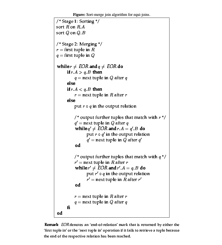
Source: http://www.dcs.ed.ac.uk/home/tz/phd/thesis/node20.htm
The crux of this algorithm is essentially the fact that it’s a linear scan on each of the two tables. Consider two “fingers” that run down the input, one for each input table. If the fingers see a pair of rows that match, then the rows get added to the output. If they don’t, then the finger pointing to the lesser value gets incremented and points at the next value. Since both inputs are sorted, this means we never miss a pair as the fingers are bound to converge on a matching pair if it exists. At the same time, this algorithm is also efficient because it “skips” values that don’t match and are irrelevant to the output. The algorithm is visualized below:

Reasons to Vectorize
While a traditional merge join algorithm is efficient in theory, it fails to take into account the overhead of integrating this algorithm into a system. Due to the nature of how data is stored and the interfaces used to process the data within the database, there are a few key factors that make this algorithm behave slower in practice than in theory.
In a database, each row of data is encoded in a format that is optimized for a specific purpose, which may not necessarily be the same purpose across all cases. To be specific, the current state of the row by row engine stores each column of every row in something called a datum. To be able to compare this datum to another datum, there is extra overhead in each call to retrieve the value, as first the type of that value has to be determined after which the value has to be decoded. Now if this process happens for every single column of every single row, it is clear that isn’t the most efficient use of processor time.
Instead, it would make sense if the type check and conversion could happen once per column, since every value in the column has the same type. This is called vectorized execution, since the idea is to operate on values a column at a time.
Constraints and Requirements
CockroachDB is currently actively working on utilizing this vectorized approach in its operators, so an interface for the vectorized model has been set up. This implies there are several constraints on how an operator can be built.
The first and most important constraint is that the vectorized merge join operator has to adhere to the higher level idea of operating on only one column per table at a time. This is a necessary conviction to ensure that shortcuts aren’t taken and that the operator as a whole doesn’t regress back to the row by row model where values of an arbitrary column can be accessed at any time.
The next constraint on the operator is that it has to adhere to the interface and properties of the other vectorized operators. This means being able to support batching, which is the process of taking large tables of input and breaking them into batches of rows, typically 1024 rows long. Each of these batches is accompanied by a null bitmap which indicates which rows are null and a selection vector. The selection vector is similar to the bitmap in that it indicates which rows are actually in the batch. This allows the flow of the operators to delay coalescing the values returned by each successive operator, saving time.
The merge join operator also has the requirement that it works for all the use cases of a typical join operator. In other words, there has to be support to:
join two tables on one or more equality columns
join on different types (ex: integers, floats, decimals, booleans, etc)
handle different types of joins (inner, outer, left, anti, semi joins, etc)
gracefully handle `COUNT` queries when there is no output
Lastly, the operator must be generally correct in that it doesn’t produce the wrong output, it is more efficient than the current row by row approach and that the code is maintainable regardless of the computation complexity.
Design Choices
While there were several iterations of the vectorized merge join operator, there were a few design decisions that ended up being essential in the formation of the operator.
The first of these decisions was the need for an explicit probing and building phases. In a traditional merge joiner, the output is generated on the fly as input rows are processed since all the columns are available at once. This is not the case in a vectorized merge joiner, as we are only able to work on one column at a time and there can be multiple columns on which we have to perform equality checks.
Thus, the merge joiner is split into a probe phase and build phase. In the probe phase, we determine all the groups that need to be materialized to output. A group is defined to be a pair of ordinal ranges, one ordinal range for each input table, such that the equality columns in each of the ranges are equivalent. In the build phase, we take these groups and materialize them a column at a time, which is a non obvious conversion from row by row to column at a time operators. Finally, each of these phases benefits from code templating, which is a technique that provides for efficient, yet readable code.
Probing for Cardinality
In a traditional merge joiner, each row is compared once, since we have access to all the columns at any point in time. In vectorized execution, we instead have to compare each column once, but determining if two rows match is dependent on all the equality columns in a row. Thus, translating the equality comparisons to vectorized execution requires saving state about the rows we are interested in. This state ends up boiling down to a list of groups for each batch, as this list of groups can be generated efficiently using an iterative approach.
To generate the list of groups, we can use a filter approach, where we first start off with the maximal match between the batches. Then, we use each equality column to filter out the rows that don’t match in each of the groups from the previous iteration. With this approach, we can effectively ignore all the extraneous information about the table and focus only on the ordinal ranges that need to be materialized.
This approach addresses the first constraint of only being able to look at one column at a time, as metadata flows between columns through the additional state about groups instead of having to index into each column for each row. Further, it also addresses points a) about joining two tables on multiple equality columns, and point b) about being agnostic to typing within the columns, since the ordinal ranges in the groups have no need for type information.
Materializing Output
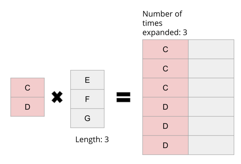
Materializing output in the merge join operator involves taking the groups/ordinal range information from the probing phase, and creating the output cross product for each group. A cross product for two input tables is defined as a new table that pairs every row of one input with every row of the other:

This cross product is intuitive to construct in a row by row fashion: create two nested loops that create every pair rows one by one and add those to the output. The interesting part is that the cross product can also be created in a column by column fashion with a key realization.
Looking at the result of the cross product, there are some patterns in the output form that can be exploited to increase performance of materialization. In the example above, it's clear that the left column of the output seems to be an “expansion” of the left input, and the right column of the output seems to be a “repetition” of the right input. A key observation is that the expansion/repetition information is actually encoded in the opposite input’s length! Thus, if you have a pair of inputs and both of their lengths, you can actually materialize the cross product in a column by column fashion:

Making use of column at a time materialization has several impacts, the most important one being performance. Materialization is one of the bottlenecks in any join operator, since copying values from the input to the output is a relatively expensive process. This means that by materializing the output column by column, we can get a significant performance boost over the traditional approach, as we don’t need to perform type inference before we copy each value. Further, this approach also satisfies the constraints of making use of the null and selection vector, as this additional information can be evaluated during the build phase, making it a good point at which to coalesce the data. The build phase addresses point c) since supporting different types of joins can then be handled exclusively by the build phase, and d) since the build phase can be skipped in its entirety if the query is a `COUNT` and there is no output.
Templating as an Optimization
Choosing to template code is a design decision that allows for more readable and maintainable code, since it provides two views to the same logic: one that is human friendly and one that is machine friendly.
Templating was originally designed for static web pages with dynamic elements. Imagine a welcome screen after a user logs in; most of the content on the web page is static, except for a few elements like the username for example. Templating involves using special syntax to allow for certain fields to be interpolated in a larger document, like the username in the webpage. It becomes interesting when the same templating construct can be used to generate source code. This can be desirable in a few cases when efficiency is a primary concern. Take into consideration the following code example:
for i := range src {

    if len(src) > 5 {

        dest[i] = src[i]

     } else {

dest[i] = src[foo[i]]

     }

}
While this may get the job done, there are obviously some inefficiencies in the fact that every iteration of the inner loop checks a property that doesn’t change for the duration of the loop. Optimizing this code would involve moving that check out of the inner loop:
if len(src) > 5 {

   for i := range src {

         dest[i] = src[i]

   }

} else {

   for i := range src {

         dest[i] = src[foo[i]]

   }

}
However, the problem with this code is that it violates the DRY (Do Not Repeat Yourself) principle which renders it unmaintainable, especially if the for loops grow in size or start diverging.
The solution in this case is templating, since most of the for loop in the example stays the same, and only the element being indexed changes. The idea with templating is that we treat the source code like a string, and so the `[i]` index can be easily swapped out for `[foo[i]]`! Thus, the templated code would look like the following:
{{ define forLoop }}

for i := range src {

      dest[i] = src[_SRC_INDEX]

}

{{ end }}

if len(src) > 5 {

     _FOR_LOOP(false)

} else {

     _FOR_LOOP(true)

}
This block of code would then be expanded out to become the optimized snippet we saw before, as the `_FOR_LOOP` would be replaced or “copy/pasted” in a sense.
This technique is useful in the merge joiner since it can be used to deal with various states of selection vector or types. Since the selection vector and type information is relevant to the column as a whole, we can perform the switching necessary to accommodate the state outside of the tight loop, similar to the technique described in the example above. Although understanding templated code has a bit of a learning curve, this technique satisfies the criteria of both efficiency and readability/maintainability.
The End Result: 3x Improvement on Standard Merge Joins
The vectorization of the merge join operator has a few key impacts on CockroachDB.
Firstly, it brings the vectorized execution engine one operator closer to being production ready, as it is currently held under an experimental/beta flag. Second, when the operator is planned and invoked, it provides a significant speed improvement over the existing row by row based model. In fact, we can see up to a 20x improvement in end to end latency for `COUNT` queries involving joins and a 3x improvement for standard merge joins:
root@:26257/tpch> set experimental_vectorize=off; # Use the row by row merge joiner

root@:26257/tpch> SELECT COUNT(*) FROM partsupp INNER MERGE JOIN lineitem ON ps_suppkey = l_suppkey INNER MERGE JOIN supplier ON s_suppkey = ps_suppkey;

...

Time: 1m54.55565s

root@:26257/tpch> SELECT ps_suppkey FROM partsupp INNER MERGE JOIN lineitem ON ps_suppkey = l_suppkey INNER MERGE JOIN supplier ON s_suppkey = ps_suppkey LIMIT 100000000;

...

Time: 31.135729s

root@:26257/tpch> set experimental_vectorize=on; # Use the vectorized merge joiner

root@:26257/tpch> SELECT COUNT(*) FROM partsupp INNER MERGE JOIN lineitem ON ps_suppkey = l_suppkey INNER MERGE JOIN supplier ON s_suppkey = ps_suppkey;

...

Time: 6.072681s

root@:26257/tpch> SELECT ps_suppkey FROM partsupp INNER MERGE JOIN lineitem ON ps_suppkey = l_suppkey INNER MERGE JOIN supplier ON s_suppkey = ps_suppkey LIMIT 100000000;

...

Time: 11.286102s
Because of this, the bottleneck becomes not the joiner itself but the speed at which data can be read from the disk. This is still important as a more optimized merge joiner can free up CPU cycles to be used elsewhere, on another query perhaps.
Want to help us build that even further optimized merge joiner? We're hiring! Check out our careers page for more information.
This post was written by George Utsin, a former Cockroach Labs intern.