Even in the 80’s, before Facebook knew everything there was to know about us, we as an industry had vast reams of data we needed to be able to answer questions about. To deal with this, data analysts were starting to flex their JOIN muscles in increasingly creative ways. But back in that day and age, we had neither machine learning nor rooms full of underpaid Excel-proficient interns to save us from problems we didn’t understand; we were on our own.
We saw in the previous post how to think about a join ordering problem: as an undirected graph with a vertex for each relation being joined, and an edge for any predicate relating two relations. We also saw the connectivity heuristic, which assumed that we wouldn’t miss many good orderings by restricting ourselves to solutions which didn’t perform cross products.
It was discussed that in a general setting, finding the optimal solution to a join ordering problem is NP-hard for almost any meaningful cost model. Given the complexity of the general problem, an interesting question is, how much do we have to restrict ourselves to a specific subclass of problems and solutions to get instances which are not NP-hard?
The topic of our story is the IKKBZ algorithm, and the heroes are Toshihide Ibaraki and Tiko Kameda. But first, we need to take a detour through a different field. We will eventually find ourselves back in JOIN-land, so don’t fear, this is still a post about databases.
Maximize Revenue, Minimize Cost
Operations research is a branch of mathematics concerned with the optimization of business decisions and management, and it has led to such developments as asking employees “what would you say you do here?”.
One sub-discipline of operations research is concerned with the somewhat abstract problem of scheduling the order in which jobs in a factory should be performed. For example, if we have some set of tasks that needs to be performed to produce a product, what order will minimize the business’s costs?
The 1979 paper Sequencing with Series-Parallel Precedence Constraints by Clyde Monma and Jeffrey Sidney is interested in a particular type of this problem centered around testing a product for deficiencies. They have a sequence of tests to be performed on the product, some of which must be performed before others. The paper gives the example of recording the payments from a customer before sending out their next bill, in order to prevent double billing - the first task must be performed before the second.
The kind of problem Monma and Sidney cover is one where these tests (henceforth “jobs”) and the order they must be performed in can be laid out in a series of parallel “chains”:
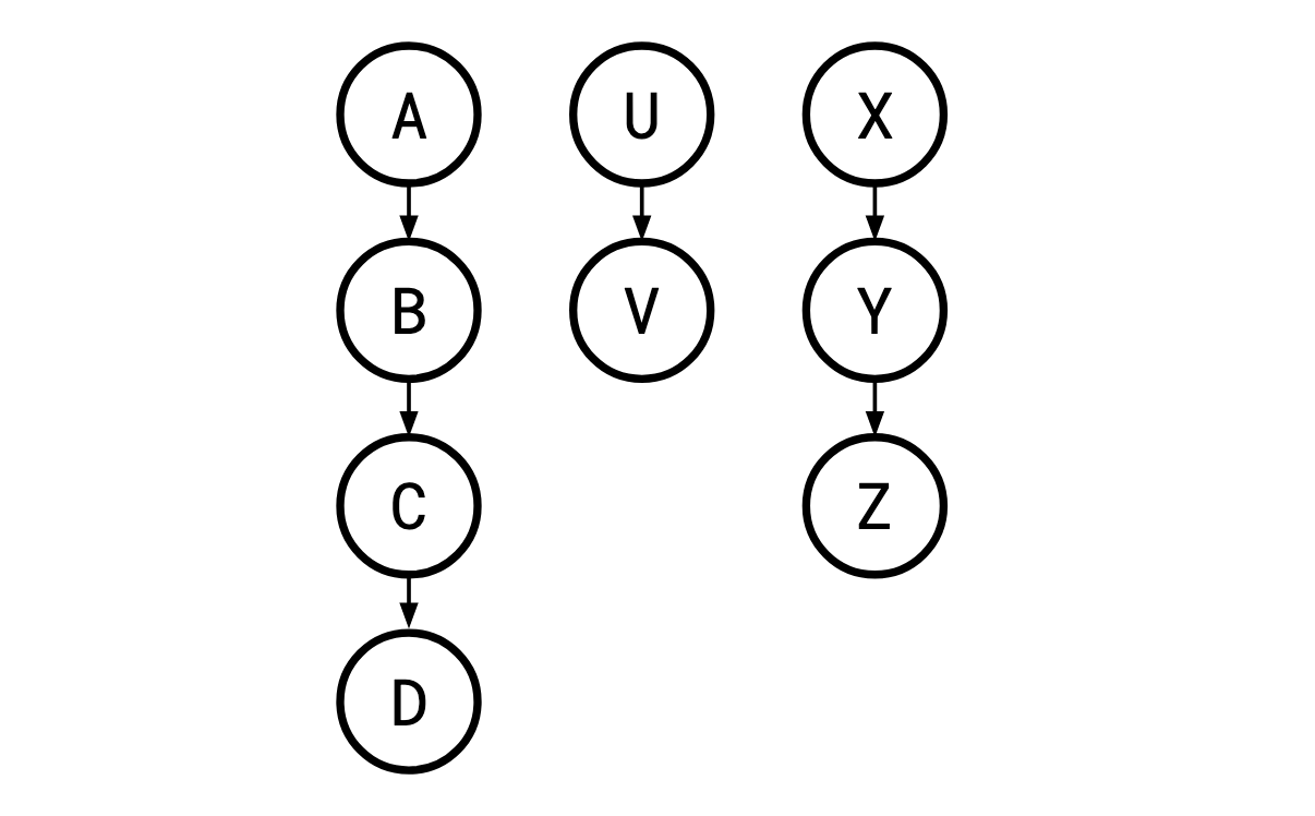
Where a legal order of the jobs is one in which a job’s parent is carried out before it is, so X,A,B,U,C,V,D,Y,Z is a legal execution here, but A,C,… is not, since B must occur before C. Such restrictions are called sequencing constraints.
This is a specific case of the more general concept of a precedence graph. A precedence graph can just be any directed acyclic graph, so in the general (non-Monma/Sidney) case, such a graph could look like this:

In the paper’s setting, each “job” is a test of a component to see if it’s defective or not. If the test fails, the whole process is aborted. If it doesn’t, the process continues. Each test has some fixed probability of failing. Intuitively, the tests we do first should have high probability of detecting a failure, and a low cost: if a test is cheap and has a 99% chance of determining that a component is defective, it would be bad if we did it at the very end of a long, expensive, time-consuming process.
Next, a job module in a precedence graph is a set of jobs which all have the same relationship to every job not in the module. That is, a set of jobs J is a job module if every job not in J either
must come before every job in J ,
must come after every job in J, or
is unrestricted with respect to every job in J
according to the problem’s precedence constraints.

For instance, in this example, {B,C}, {X,Y,Z}, and {V} are job modules, but {X,Z} is not a module because Y must come before Z, but is after X. Similarly, {A,U} is not a module because V must come after U but is unrestricted relative to A.
When we use j to represent an object, we’re talking about one single job, and when we use sand t, we’re talking about strings of jobs, as in, =12…s=j1j2…jn, which cannot be further split apart, and are performed in sequence. In general, these are somewhat interchangeable. In this setting, jobs are just strings of length one.
If two strings are in a module together, we can concatenate them in some order to get a new string. Since the constituent jobs and strings are in a module (and thus have all the same constraints), there’s only one natural choice of constraints for this new string to have. It’s generally easier to reason about a problem with fewer jobs in it, so a desirable thing to be able to do is to concatenate two jobs to get a new, simpler problem that is equivalent to the original one. One of the key challenges we’ll face is how to do this.
We use (1,2,…)f(s1,s2,…) to refer to the cost of performing the string 1s1, followed by the string 2s2, and so on (think of this function as “flattening” of the sequences of jobs). ()q(s) is the probability of all of the tests in ssucceeding. We assume all the probabilities are independent, and so the probability of all of the jobs in a string succeeding is the product of the probability of success of each individual job. If the sequencing constraints constrain a string sto come before a string t, we write →s→t(read “scomes before t”). We’re going to use strings to progressively simplify our problem by concatenating jobs into strings.
The expected cost of performing one sequence of jobs followed by another sequence of jobs is the cost of performing the first sequence plus the cost of performing the second sequence, but we only have to actually perform the second sequence if the first sequence didn’t fail. Thus, in expectation, the cost is (,)=()+()()f(s,t)=f(s)+q(s)f(t).
Since this is recursive, we need a base case, and of course, the cost of performing a single job is simply the cost of the job itself: ()=f(j)=cj. An important property of this definition is that f is well-defined: (1,2)=(1′,2′)f(S1,S2)=f(S1′,S2′) whenever 12=1′2′S1S2=S1′S2′(verifying this is left as an exercise).
An adjacent sequence interchange is a swap of two adjacent sequences within a larger sequence:

This is an adjacent sequence interchange of ,,X,Y,Z with ,U,V.
A rank function maps a sequence of jobs 12…j1j2…jnto a number. Roughly, a rank function captures how desirable it is to do a given sequence of jobs early. ()<()r(s)<r(t) means we would like to do sbefore t. A cost function is called adjacent sequence interchange (ASI) relative to a rank function r if the rank function accurately tells us when we want to perform interchanges:
(,,,)≤(,,,)if ()≤()f(a,s,t,b)≤f(a,t,s,b) if r(s)≤r(t)
And a cost function f is ASI if there exists a rank function it is ASI relative to. I’m sure you’ll be shocked to learn the f we derived above ((,)=()+()()f(s,t)=f(s)+q(s)f(t)) is ASI.
Note that even though we may have a rank function which tells us we would like to do a given sequence of jobs early, the sequencing constraints might prohibit us from doing so.
The ASI theorem (Monma and Sidney call this “Theorem 2”, but we’re going to use it enough for a real name) mildly paraphrased:
Let f be ASI with rank function r, and let sand tbe strings. Consider a job module {,}{s,t} in a general precedence graph, where →s→tand ()≤()r(t)≤r(s). Then there is an optimal permutation with s immediately preceding t.
Let’s break down this theorem. First of all, note that it applies to a general precedence graph. This means we’re not restricting ourselves to the “parallel chains” kind of graph described above.
s→t means s must come before t(s and t are already strings in the current iteration of our problem, and they inherit the constraints of the jobs they are composed of). However, r(t)≤r(s) means we would like to put t before s. What this theorem is saying is that in this scenario, we’re not forgoing optimality by ordering s immediately before t. This is very useful, because it allows us to take two strings, s and t, and replace them with the new string st which is their concatenation. Importantly, this is saying that there is an optimal permutation with s immediately preceding t, not that in any every optimal permutation this is the case. The proof of this theorem is pretty simple so I’ve included it.
Proof of the ASI theorem: Every optimal permutation looks like ⟨u,s,v,t,w⟩ since s→t. If v is empty, we’re done. otherwise, if r(v)≤r(s), then by ASI we can swap s and v without dropping the cost to get ⟨u,v,s,t,w⟩. If r(s)<r(v), then by transitivity r(t)<r(v) and again by ASI we can swap v and t without dropping the cost to get ⟨u,s,t,v,w⟩. These swaps must be legal since {s,t} is a job module.
Finally, our friends Monma and Sidney describe the parallel chains algorithm. It goes like this:
If, for every pair of strings s and t , s → t implies r( s )<r( t ) (meaning that the constraints and the rank agree about the correct order for the two), go on to step 2. If the two relations disagree somewhere, then we can find a job module { s , t } for which they disagree [1]. Then, by the ASI theorem, we can concatenate s and t into the sequence s t (since we know there’s some optimal solution where they’re adjacent), which we then treat as a new string. Now repeat step 1. Our problem has exactly one less string in it now, so this process can’t go on forever.
Sort the remaining strings by their value under r. Since step 1 terminated, the resulting order is legal, and since f is ASI, it’s optimal.
The core idea of the algorithm is that we’d like to just blindly order all the jobs by their value under the rank function, but situations where the rank function and the precedence constraints disagree prohibit that. The ASI theorem gives us a tool to eliminate precisely these scenarios while keeping access to optimal solutions, so we repeatedly apply it until we are free to simply sort.
Back to Databases
Back to the topic of Join Ordering. For their paper “On the Optimal Nesting Order for Computing N-Relational Joins,” Toshihide Ibaraki and Tiko Kameda were interested in instances of the join ordering problem for which
solutions were restricted to those that
were left-deep and
contained no cross products
the only join algorithm used was the nested-loop join, and
the query graph was a tree.
As we saw before, a plan is left-deep if the right input to every join operator is a concrete relation, and not another join operation. This gives a query plan that looks something like this, with every right child being a “base relation” and not a join:

and not like this, where a join’s right child can be another join:

Since the shape of the plan is fixed, we can talk about the plan itself simply as a sequence of the relations to be joined, from left to right in the left-deep tree. We can take a query plan like this:

and represent it like this:

When we say that the query graph must be a “tree”, we mean in a graph theoretical sense—it’s a graph that is connected and has no cycles. If you primarily identify as a computer science person and not a mathematician, when you hear “tree” you might picture what graph theorists call a “rooted” tree. That is, a tree with a designated “special” root vertex. It’s like you grabbed the tree by that one designated vertex and let everything else hang down.
Here’s a tree:

Here it is rooted at A:

Here it is rooted at D:

This distinction is important for our purposes because it’s easy to get a rooted tree from an unrooted tree: you just pick your favourite vertex and call it the root.

Query graphs and query plans are fundamentally different. The query graph describes the problem and a query plan the solution. Despite this, they’re related in very important ways. In a left-deep query plan, the relation in the bottom-left position is quite special: it’s the only one which is the left input to a join. If we are obeying the connectivity heuristic (no cross products), this gives us a way to think about how exactly it is we are restricted.
In the plan above, A and B must share a predicate, or else they would cross-product with each other. Then C must share a predicate with at least one of A or B. Then D must share a predicate with at least one of A, B, or C, and so on.
Let’s assume for a second that given a query graph, we know which relation will wind up in the bottom-left position of an optimal plan. If we take this special relation and make it the root in our query graph, something very useful happens.
Given our rooted query graph, let’s figure out what a plan containing no cross products looks like. Here’s an example of such a rooted query graph:

Since we must lead with A, which vertices can we then add to get a legal ordering? Well, the only three that don’t form a cross product with A are B, C, and D. Once we output, C, it becomes legal to output F, and so on. As we go down the tree, we see a necessary and sufficient condition for not introducing cross products is that the parent of a given relation must have already been output. This is effectively the same as the precedence constraints of the job-scheduling problem!
Of course, beforehand, we don’t know which relation will be the optimal one to place in the bottom left. This is going to turn out to be only a minor problem: we can just try each possible relation and choose the one that gives us the best result.
So, from here on, we’ll think of our query graph as a rooted tree, and the root will be the very first relation in our join sequence. Despite our original graph having undirected edges, this choice allows us to designate a canonical direction for our edges: we say they point away from the root.
A Tale of Two Disciplines
I can only imagine that what happened next went something like this:
Kameda sips his coffee as he ponders the problem of join ordering. He and Ibaraki have been collaborating on this one for quite a while, but it’s a tough nut to crack. The data querying needs of industry grow ever greater, and he has to deliver to them a solution. He decides to take a stroll of the grounds of Simon Fraser University to clear his mind. As he locks his office, his attention is drawn by the shuffling of paper. A postdoc from the operations research department is hurrying down the hall, an armful of papers from the past few years tucked under her arm.
Unnoticed, one neatly stapled bundle of papers drops to the floor from the postdoc’s arm. “Oh, excuse me! You dropped—” Kameda’s eyes are drawn to the title of the paper, Sequencing With Series-Parallel Precedence Constraints, as he bends down to pick it up.
“Oh, thank you! I never would have noticed,” the postdoc says, as she turns around and reaches out a hand to take back the paper. But Kameda can no longer hear her. He’s entranced. He’s furiously flipping through the paper. This is it. This is the solution to his problem. The postdoc stares with wide eyes at his fervor. “I…I’ll return this to you!” He stammers, as he rushes back to his office to contact his longtime collaborator Ibaraki.
If this isn’t how it happened, I’m not sure how Ibaraki and Kameda ever made the connection they did, drawing from research about a problem in an entirely different field from theirs. As we’ll see, we can twist the join ordering problem we’re faced with to look very similar to a Monma-and-Sidney job scheduling problem.
Recall that the selectivity of a predicate (edge) is the amount that it filters the join of the two relations (edges) it connects (basically, how much smaller its result is than the raw cross product):
sel(p)=∣A×B∣∣A⋈pB∣ Designating a root allows us another convenience: before now, when selectivity was a property of a predicate, we had to specify a pair of relations in order to say what their selectivity was. Now that we’ve directed our edges, we can define a selectivity for a given relation (vertex) as the selectivity of it with its parent, with the selectivity of the root being defined as 1. So in our graph above, we define the selectivity of H to be the selectivity of the edge between F and H. We refer to the selectivity of R by fR.
This definition is even more convenient than it first appears; we’re restricted by the precedence constraints already to include the parent of a relation before the relation itself in any legal sequence, thus, by the time a relation appears in the sequence, the predicate from which it derives its selectivity will apply. This allows us to define a very simple function which captures the expected number of rows in a sequence of joins. Let ∣Ni=∣Ri∣, then for some sequence of relations to be joined S, let T(S) be the number of rows in the result of evaluating S. Then:
T(Λ)=1 for the empty sequence ΛΛ, since the “identity” relation is that with no columns and a single row, and T(S)=fRi1Ni1fRi2Ni2…fRikNik for S=Ri1Ri2…Rik T(S) is simply the product of all the selectivities and the sizes of the relations contained within it. This follows directly from the definition of selectivity from the first post and the precedence constraints.
Further, to evaluate how good a query plan is, we need to have a cost model that tells us how expensive it is to execute.
Intuitively, the cost of executing a sequence of joins is
the cost of executing a prefix of the joins, plus
the cost of executing the rest of the joins by themselves, times the number of rows in the prefix (since we’re doing a nested-loop join).
This gives us this recursive definition of the cost function for a sequence:
C(Λ)=0 for the empty sequence ΛΛ, C(Ri)=fRiNifor a single relation Ri, C(S1S2)=C(S1)+T(S1)C(S2) for sequences of relations S1and S2.
Again, things are looking very similar to the world of Monma and Sidney. We can even define a rank function for this setting to be
r(S)=C(S)T(S)−1.
Recall the property we want of a rank function in order for f to be ASI. We want it to be the case that:
C(AS2S1B)≤C(AS1S2B) if r(S2)≤r(S1)
Through some opaque algebra, we can see this is true (don’t worry too much about following this, you can just trust me that it shows that f is ASI):
C(AS1S2B)=C(AS1)+T(AS1)C(S2B)=C(A)+T(A)C(S1)+T(A)T(S1)[C(S2)+T(S2)C(B)].
Thus, C(AS1S2B)−C(AS2S1B)=T(A)[C(S2)(T(S1)−1)−C(S1)(T(S2)−1)] =T(A)C(S1)C(S2)[r(S1)−r(S2)].
And so C(AS1S2B)−C(AS2S1B) is negative precisely when r(S1)−r(S2) is. □□
(As an aside, I don’t have a good intuitive interpretation of what this particular rank function represents—this is one of those cases in math where I note that the algebra works out on paper and then promptly start treating r(S) as a black box.)
We’re nearly there. However, we can’t apply the parallel chains algorithm, because our query graph might not be a parallel chain graph (it’s a rooted tree). How we’re going to approach this is by iteratively applying “safe” transformations to the query graph until it becomes a single chain. We do this by looking for wedges. A wedge is two or more chains joined at a vertex:
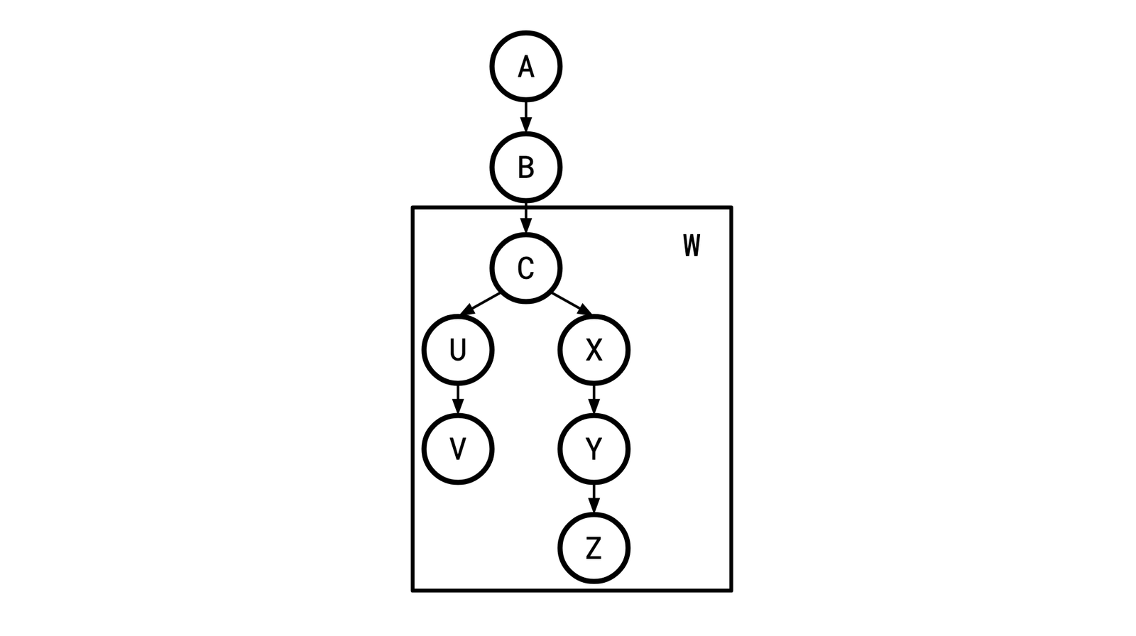
W here is a wedge, and C is the “root” of W.
Note that wedges are precisely the structure that make our graph not a chain, so if we can eliminate one, we can bring ourselves closer to a chain.
Ibaraki and Kameda first define a process they call NORMALIZE(S) (…it was the 80s. That was how algorithm names were written), where S is one chain of a wedge:
While there is a pair of adjacent nodes S 1 and S 2 with S 1 followed by S 2 in S, such that r(S 1 )>r(S 2 ):
find the first such pair (starting from the beginning of S) and replace S 1 and S 2 by a new node S 1 S 2 , representing a subchain S 1 followed by S 2.
Here’s an example of applying NORMALIZE:
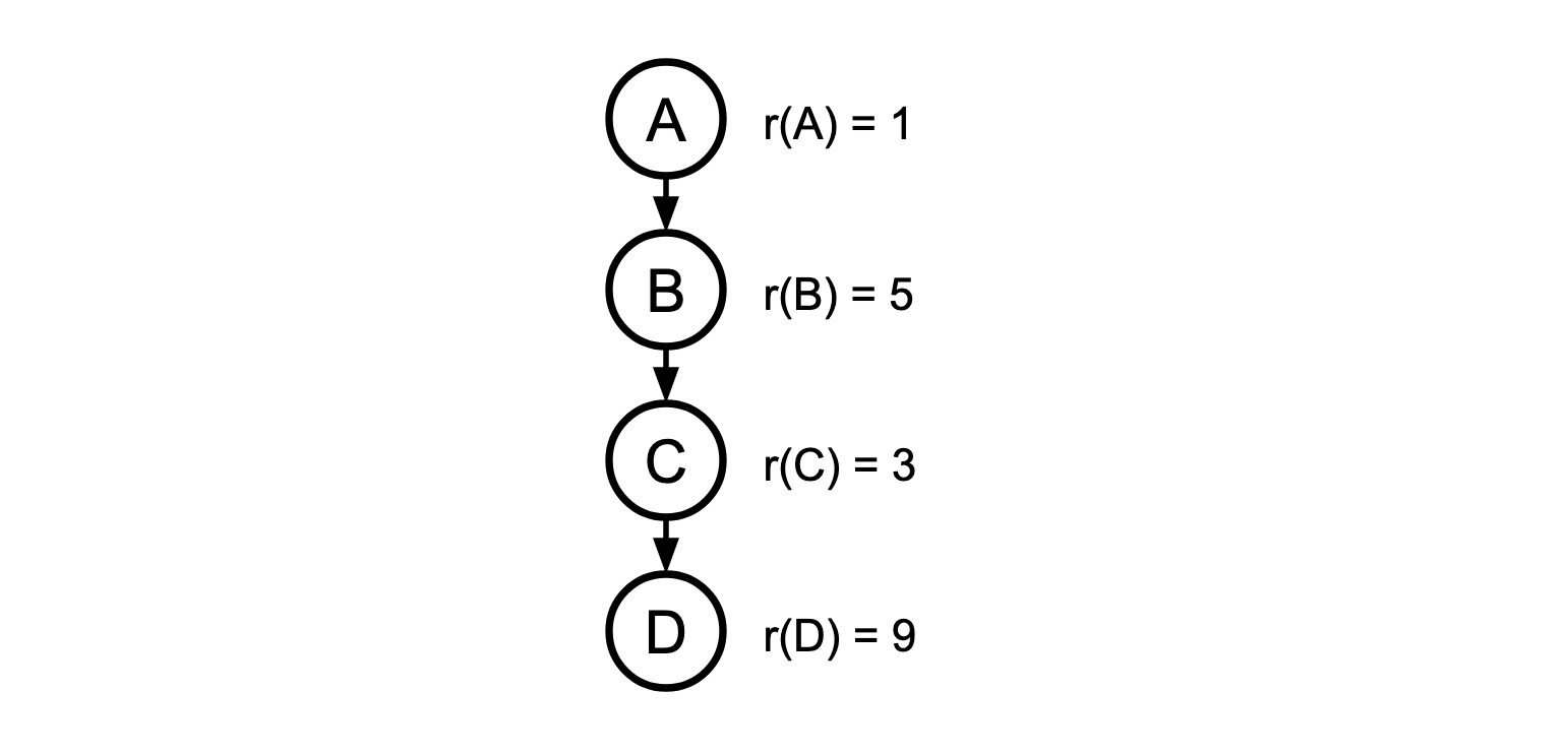
In this chain, B and C are such a pair of misordered nodes. Applying NORMALIZE, we get a new node, BC, with a new rank:

This is the same as the trick pulled in the parallel chains algorithm: the ASI theorem guarantees that by performing this merging operation we don’t lose access to any optimal solutions.
Once the chains in W are completely normalized (meaning they’re ordered by their value under the rank function) we can merge them into a single chain which maintains that ordering. Any interleaving of them is legal, since they’re unrelated by any precedence constraints. We then continue this process of eliminating wedges until there are none left, and we are left with the optimal ordering.
The process of eliminating all the wedges in a tree can be done in time O(nlogn), but there’s a catch! Since we rooted our tree by picking an arbitrary vertex before, this solution is only guaranteed to be optimal for that particular choice of vertex. The fix is easy: we perform the algorithm for every choice of starting vertex and take the best one. Running the algorithm for a single choice of root takes O(nlogn) to run, and so performing it for every choice of root takes O(n2logn). This is the algorithm and runtime that Ibaraki and Kameda presented in their paper.
My queries are still taking too logn!
There’s one final piece to fall into place to get the final IKKBZ algorithm. The IK in IKKBZ indeed stands for Ibaraki and Kameda. At VLDB 1986, Ravi Krishnamurthy, Haran Boral, and Carlo Zaniolo presented their paper Optimization of Nonrecursive Queries. Check out this glorious 1986-era technical diagram from their paper:

Their trick is that if we pick A as our root and find the optimal solution from it, and then for our next choice of root we pick a vertex B that is adjacent to A, a lot of the work we’ll have to do to solve from B will be the same as the work done from A.
Consider a tree rooted at A:

(Where X is all the nodes that live beneath A and Y is all the nodes that live beneath B) and say we have the optimal solution S for the A tree. We then we re-root to B:

KB&Z recognized that the X and Y subtrees in these two cases are the same, and thus when we eliminate all the wedges beneath A and B, the resulting chains will be in the same order they were in for the tree rooted at A, and this order is the same as the order implied by S. So we can turn the X and Y subtrees into chains by just sorting them by the order they appear in S.
This means that we can construct the final chains beneath A and B without a O(nlogn) walk, using only O(n) time to merge the two chains, so in aggregate, we do this for every choice of root, and arrive at a final runtime of O(n2).
OK, let’s take a step back. Who cares? What’s the point of this algorithm when the case it handles is so specific? The set of preconditions for us to be able to use IKKBZ to get an optimal solution was a mile long. Many query graphs are not trees, and many queries require a bushy join tree for the optimal solution.
What if we didn’t rely on IKKBZ for an optimal solution? Some more general heuristic algorithms for finding good join orders require an initial solution as a “jumping-off point.” When using one of these algorithms, IKKBZ can be used to find a decent initial solution. While this algorithm only has guarantees when the query graph is a tree, we can turn any connected graph into a tree by selectively deleting edges from it (for instance, taking the min-cost spanning tree is a reasonable heuristic here).
The IKKBZ algorithm is one of the oldest join ordering algorithms in the literature, and it remains one of the few polynomial-time algorithms that has strong guarantees. It manages to accomplish this by being extremely restricted in the set of problems it can handle. Despite these restrictions, it can still be useful as a stepping stone in a larger algorithm. Adaptive Optimization of Very Large Join Queries has an example of an algorithm that makes use of an IKKBZ ordering as a jumping off point, with good empirical results. CockroachDB doesn’t use IKKBZ in its query planning today, but it’s something we’re interested in looking into in the future.
Appendix
Sketch of a proof of [1]: Since the two are related by the precedence constraints, they’re in the same chain. If they’re not adjacent in that chain, there’s some x in between them, so s→x→t. If r(x)<r(t), then {x,t} is a “closer” bad pair. If r(x)≥r(t) then {x,s} is a “closer” bad pair. Then by induction there’s an adjacent pair.