

In this post, I’ll skim the surface of a very common pattern in application development: full text indexing and search. I’ll start with a bit of motivation, what prompted me to explore this using CockroachDB. Next, I’ll introduce the initial pass at a solution, followed by a deeper explanation of how that was done, and I’ll then improve on that result by adding a “score”. Finally, I’ll discuss the limitations of this simplistic approach, within the context of information retrieval, ending with my answer to “So, why’d you do it?” Let’s get started.
The Experiment: Build Full Text Indexing with CockroachDB
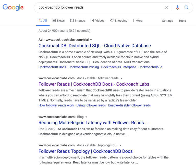
Yesterday, after becoming intrigued by the idea of “follower reads” in CockroachDB, I used Google’s search to help me find material on this topic. In the ranked search results, shown below, note the order: the “Follower Reads ...” one is first (after the ad), then there is a blog post and, finally, the one beginning “Follower Reads Topology”.
Naturally, my mind drifted and I speculated about how I might attempt to implement a text search feature using the very technology which was the subject of my search: CockroachDB. As we know, CockroachDB is a horizontally scalable, geographically distributed, ACID compliant database optimized for OLTP workloads; still, I was curious to see how it would handle this analytic use case. Well, as it turns out, it’s a tractable problem, more so if you skip building the nice UI and other amenities. The image below depicts my initial foray into this realm. It’s a screenshot of my DbVisualizer window, where I ran the equivalent of the Google search shown above, though here my data set was restricted to the docs for v20.2 of CockroachDB. What I find encouraging about this is (1) the top two results match those from the Google search and (2) the query returned results in under 40 ms.
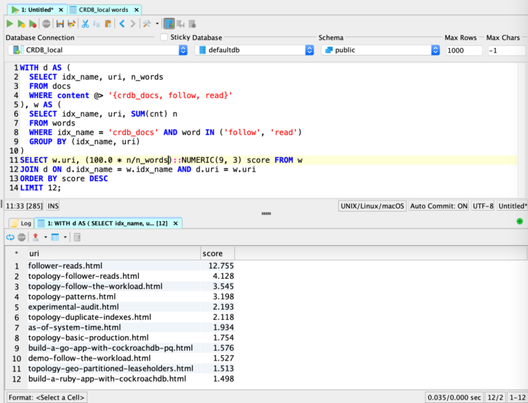
I should probably explain what’s going on within that DbVisualizer window. Overall, this is a SQL query which blends the results of two separate queries, using a common table expression (CTE), ultimately yielding a sorted list of search results. In the top query, on lines 2 - 4, the goal is to find the rows of the “docs” table where the content column contains the given three terms: “crdb_docs”, “follow”, and “read”. That is achieved is through the use of the “@>” operator, which ensures that the query optimizer chooses the inverted index (aka Generalized Inverted Index, or “GIN”) on the content column, thus speeding things up. All by itself, this initial query (labeled “d” here) provides an unordered list of search results. Not too shabby. Here’s what this initial query looks like:
SELECT idx_name, uri, n_words
FROM docs
WHERE content @> '{crdb_docs, follow, read}';
Let me back up just a bit. To get to this point, I had to spin up a local CockroachDB cluster, create two tables, index certain columns within these tables, then load my HTML data into them. Here's a link on how to spin up CockroachDB cluster, and I’ll include my DDL, here:
CREATE TABLE docs
(
  idx_name TEXT
  , uri TEXT
  , content TEXT[]
  , n_words INT
  , PRIMARY KEY (idx_name, uri)
);

CREATE TABLE words
(
  idx_name TEXT
  , uri TEXT
  , word TEXT
  , cnt INT
);

-- Secondary indexes
CREATE INDEX ON docs USING GIN(content);
CREATE INDEX ON words (idx_name, word) STORING (cnt);
As thrilled as I was with these initial results, based solely on the “d” query, the novelty wore off pretty quickly. Missing from this was some kind of ranking mechanism, to order the results in descending order of relevance. That’s where the query marked “w” comes in. This one runs against a “words” table that tracks the total number of occurrences of each word, in each of the documents (and, in each “index”, since I anticipated there being more than one index). This query computes an aggregate, by combining SUM with GROUP BY. On line 11, elements from both queries are combined to generate a normalized score for each of the search results. This is where the CTE comes in handy, since it enables me to compute that aggregate in query “w” and later refer to it in the score computation. Finally, on line 13, the search results are sorted in descending order, by score. Here’s the final query, featuring the CTE:
WITH d AS (
  SELECT idx_name, uri, n_words
  FROM docs
  WHERE content @> '{crdb_docs, follow, read}'
), w AS (
  SELECT idx_name, uri, SUM(cnt) n
  FROM words
  WHERE idx_name = 'crdb_docs' AND word IN ('follow', 'read')
  GROUP BY (idx_name, uri)
)
SELECT w.uri, (100.0 * n/n_words)::NUMERIC(9, 3) score FROM w
JOIN d ON d.idx_name = w.idx_name AND d.uri = w.uri
ORDER BY score DESC
LIMIT 12;
Now for the inevitable “limitations and disclaimers”. If you glance at the code in the GitHub repository for this little experiment, you’ll notice it’s a pretty simplistic approach to full text indexing. This is sort of the classic “bag of words” approach to information retrieval. And, it does stemming and case folding (you may have noticed the terms “follow” and “read” in the SQL query). Though this code does incorporate “term frequency” (TF), it ignores the closely related concept of “inverse document frequency” (IDF). Mitigating that is the use of a “stop word” list to help identify and remove frequently encountered words which contribute little to the meaning of the text (“the”, “a”, “an”, etc.). Since I hoped to keep the total number of words in the vocabulary reasonable, I used a list of English words and only indexed terms appearing in this list. The impact of this is that a search for “CDC” would return zero results, though a search for “change data capture” would work fine. Another shortcoming is that the “term offsets” of each of the words aren’t stored, so it’s impossible to do a phrase query. Oh, search result highlighting and/or gisting, to show the user the context within the document that triggered the “hit” in the search -- also missing here. The last thing is that this is restricted to English language texts, though it’s not hard to imagine extending it to handle other languages.
Building a successful full text indexing and search engine is quite a task. I’ve used Elasticsearch (ES) and Solr in the past, as well as Lucene, which forms the underpinnings of both ES and Solr. Using ES or Solr, you get a text index and search experience out of the box that provides all that I mentioned up above, and much more. If your goal is search, I highly recommend them; you can even use CockroachDB’s change data capture (CDC) feature to set up a change feed which will keep your Elasticsearch or Solr indexes sync’d to your CockroachDB tables.
Why Build Full Text Indexing in CockroachDB?
Having said all that, the inevitable question is “So, why’d you do it?” Two reasons: (1) I’m into text search; (2) I’d just finished some experiments with geospatial data, which uses the GIN indexes, so I thought about using them again. Also, when you have in your hands an amazing cloud-native, distributed SQL DB like CockroachDB, you’re tempted to stretch a little and see how it fares when applied to some more niche data problems. I imagine I’ll not be able to resist further experimentation with this, and I’ll update that GitHub repo as I go. Please feel free to fork or clone that and indulge your own text search yearnings. Finally, thank you very much for sticking with me on this brief foray into the topic of text search. I hope you enjoyed it.
Additional References
SQL and Python code for this experiment (GitHub repo)
Google’s stance on using images of its search product in documents
Lucene’s discussion of TF*IDF for relevance scoring