Six months ago, we reported our first implementation of SQL joins in CockroachDB. At that point in development, we merely provided a functional proof of concept that was severely limited performance-wise.
This is changing, gradually.
We are preparing to launch CockroachDB 1.0 later this spring, and SQL joins in CockroachDB 1.0 will be usable, if underpowered.
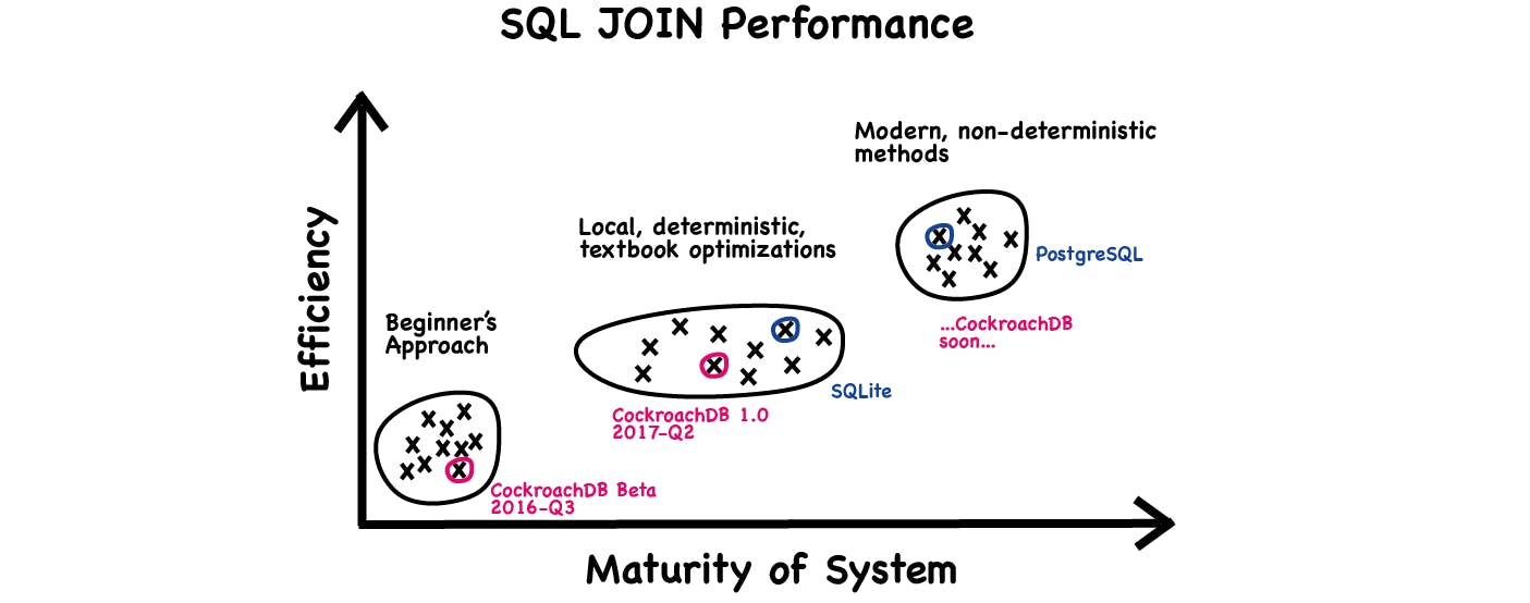
The story in the infographic above is that we are working to make SQL joins perform better than the naive code we presented in July 2016. We still have a long way to go to land in the same ball park as the more mature, enterprise-grade SQL engines, but we will get there eventually.
This blog post is meant as the next chapter of our story on joins in CockroachDB. In this chapter, you will learn how join query execution works now, what you can do now which you couldn’t do before, and what you can expect in v1.0. We’ll conclude with a peek at our roadmap on SQL optimizations.
Six months further down the road
In summary:
We have replaced our default implementation of the join operator with a hash join. This changes the asymptotic time complexity for two input tables of sizes N and M to O(N+M) in most cases instead of O(N×M) previously — a linear speedup.

Image inspiration: Time Complexity and Why It’s Important
We have done some preliminary work on filter optimization. This causes many simple joins to be simplified to a constant-time operation instead of a costly quadratic lookup like previously.
We have some preliminary working code to distribute and parallelize the execution of joins. This can enable speedups linear in the size of the cluster for some queries.
Abstract query semantics
CockroachDB interprets every SQL join as a binary operation.
SELECT statements using multiple joins are transformed to a tree of binary join operations that follow the syntax of the query, assuming the join operator is left-associative. That is:
SELECT * FROM a, b, c, WHERE ...
Is interpreted as:
SELECT * FROM ((a CROSS JOIN b) CROSS JOIN c) WHERE …
Which internally is processed like this:
                        Render *
                           |
                          Join
                        /     \
                     Join      c
                    /  \
                   a    b
This overall interpretation has not changed yet: CockroachDB currently processes the joins in the logical order specified by the query, and the user has complete control over the join order. (The flip side of this control, naturally, is that if the user does not think about the join order the result can be sub-efficient. More about this later.)
On top of this general structure for the data operands for a SELECT, CockroachDB must then filter out rows based on the WHERE clause.
Until recently, a query of the form
SELECT * FROM abc WHERE abc.x > 3 AND abc.y < 2
Would be handled as:
Render *
   |
Filter on abc.x > 3 AND abc.y < 2
   |
  abc
Which means that in combination with joins we had the following situation: a query with the form
SELECT *
  FROM a, b, c
 WHERE a.x = b.x AND b.y = c.y AND a.x+b.y+c.z > 0
Was handled like this:
                    Render *
                      |
                Filter on a.x = b.x AND b.y = c.y
                          AND a.x+b.y+c.z > 0
                      |
                     Join
                   /     \
                Join      c
               /  \
              a    b
This meant that the entire cross-join result of a CROSS JOIN b CROSS JOIN c needed to be computed before we could decide which rows would be reported to the client. This could produce extremely large intermediate result sets in memory even for small input tables — e.g. a simple 5-way join between small tables with 100 rows each would produce 10 billion rows in memory before any result could be produced!
This was silly, because what was really intended by the query above is more something like:
                    Render *
                      |
                Filter on a.x+b.y+c.z > 0
                      |
                    Join on b.y = c.y
                   /               \
             Join on a.x = b.x      c
               /  \
              a    b
Processing the query like this obviously reduces the amount of intermediate rows greatly. We needed to get here somehow, and the process to get there is what we describe in the upcoming sections.
Optimizing the join operator
The first thing that we changed was how the individual binary joins are processed. Previously we used this “nested loop”, a sequential algorithm which for every incoming row on one side looks at every row on the other side to decide whether there is a match. This works but always has quadratic complexity, i.e. nearly the worst one can imagine.
So over the fall our beloved co-op and colleague Irfan Sharif provided an alternate implementation based on the classical hash join algorithm: the results of the first table are loaded in a hash table keyed with the join columns. The second table is then scanned, and at every row, the hash table is looked up to see if there is a match. The hash table lookup runs in amortized constant time, compared to the linear lookup of the initial code, and thus tremendous speedups were obtained.
Because hash joins are conceptually only defined for equijoins (joins where the result exists when two input rows are pairwise equal on the join columns), this new algorithm was initially only activated for joins defined with USING or NATURAL, where the equality mandated by the query syntax. Soon afterwards, we were able to detect equality expressions when using the ON syntax and use hash joins for them as well.
Then, an additional realization dawned: when a join is specified using a more complex expression, we can use the same hash join code by running the join “as if” there were no equality column: all the rows of the first input table then simply land in one bin of the hash table, and we must then scan the content of this table for every row of the second input table to decide join results.
This is exactly equivalent in behavior to the “nested loop” code. (Not a big surprise in hindsight though, because the theory already tells us that hash joins degenerate to quadratic complexity when there are few equality classes in the input.) So we ended up removing the original code entirely, and replacing it with hash joins everywhere, letting the hash join devolve into the original behavior when it can’t do its magic.
Side note: A common ritual among SQL database implementers is to experience trouble and discomfort while trying to make outer joins work properly. For example, PostgreSQL supported inner joins in its first release in 1996 but only started supporting outer joins in 2001. We are experiencing our fair share of hassle too, and we had to fix our outer join implementation once again. Hopefully outer joins are functional in CockroachDB but they won’t receive as much attention for optimizations until the rest of our implementation matures a bit further.
Optimizing query filters
The second thing we looked at was to reduce the strength of join operations: how many rows are provided as input to the hash join algorithm.
To do this, we observed that many queries specify a WHERE clause which narrows down the result rows, but that this WHERE clause could equally well be applied before the join instead of afterwards.
That is, a query of the form:
SELECT * FROM a,b WHERE a.x = b.x
Is equivalent to:
SELECT * FROM (a JOIN b USING(x))
And a query of the form:
SELECT * FROM a, b WHERE a.y > 3 AND b.z < 4 AND a.x = b.x
Is equivalent to:
SELECT *
   FROM (SELECT * FROM a WHERE a.y > 3) AS a
        JOIN
        (SELECT * FROM b WHERE b.z < 4) AS b
        USING (x)
To understand why this matters, imagine that tables a and b both contain 10 million rows, but only 100 rows in a have column y greater than 3 and 100 rows in b have column z smaller than 4.
In the original case, the cross join would need to load the complete left table in memory (10 million rows), which would exhaust the server memory, before it could apply the filter. If we look at the equivalent query underneath, the two filters are applied first and the inner join then only has to match 100 rows on both sides to each other — a much lighter operation.
Transforming the original query to the latter, equivalent query is an instance of a larger class of optimizations called “selection propagation”. The idea stems from relational algebra, where the various data processing stages of a SQL query are expressed as a formula using only basic building blocks like projection, selection, joins, etc. The theory explains that most queries that perform something (e.g., a join), then a selection, (a WHERE filter) can be always rewritten to do the selection first, then the rest — it is said that selection is commutative with most other relational operators — and that this transformation always reduces the strength of the other operators and is thus always desirable.
So over the last quarter of 2016, we implemented this optimization in CockroachDB, and it is now activated for (but not limited to) inner joins.
Once this was done, an immediate benefit was automatically activated too: as the WHERE filters “propagate down” the joins in the query, they become visible as constraints on the lookups from the table operands, and thus become visible for index selection and K/V lookup span generation.
Thanks to this fortuitous combination of existing optimizations, joins are now also accelerated by the ability to use indexes and point KV lookups to access the individual table operands. For example, in SELECT cust.name, order.amount FROM cust JOIN order USING(cust_id) WHERE cust_id = 123, just one K/V lookup will now be performed on cust and order, where previously all customers would be loaded in memory before the join could proceed.
Elision of unused columns
In addition to the work presented so far, which supports the bulk of the acceleration of queries compared to summer 2016, another optimization was introduced under the hood.
Suppose you work with a “customer” table with columns “name”, “address”, ”id”, “company”, and you perform a query like SELECT customer.name FROM customer, order WHERE customer.id = order.cust_id. Internally, before the optimization above apply, this query is transformed to this:
SELECT customer.name
  FROM (SELECT name, address, id, company FROM customer)
       JOIN
       (SELECT … FROM order)
 WHERE customer.id = order.id
That is, the input operand to the join “sees” all the columns in the customer table. This is necessary because the WHERE clause, which is specified “outside” of the join operator, can use any combination of columns from the input table, regardless of what the outer SELECT ends up using.
The reason why this matters is that without additional care, this query could then be translated to use a table scan on the “customer” table that retrieves all the columns semantically listed at that level. In this example, that would mean all the columns in the table — even those columns that won’t be needed in the end. Then the join operation would accumulate all this data in memory, before the contents of the second table are read in to decide the final join results, and before the outer SELECT throws away all columns but one (“name”) to produce the query’s results.
For tables that contain many columns but are used in queries that only access a few of them at a time, this behavior wastes a lot of time (loading and moving data around for nothing) and memory (to store these unneeded values) and network bandwidth.
Acknowledging that cases where tables contain many columns but queries involving joins only use a few of them are rather common, we had to care about this seriously. So we implemented a small optimization that looks at the query from the outside and determines at each level which columns are strictly necessary to produce the final results. Every column that is not necessary is simply elided, i.e., it is not loaded nor further manipulated/communicated with during the query’s execution.
Sneak peek — distributed query execution and parallelization
As announced in the previous blog post on joins, we are also working on a distributed query execution engine. The present post is not the opportunity to detail this much — we will start a series of blog posts dedicated to distributed query execution — however here is a sneak peek of how it will help with joins.
When CockroachDB distributes a join, it loads the data from both table operands simultaneously and in parallel on multiple nodes, performing multiple parts of the join on different nodes of the cluster, before merging the results towards the node where the query was received from the client. This way, the join can be theoretically sped up by a factor linear in the size of the cluster (in the ideal case).
Again, we will report more on this topic separately! The update here is that this code is now available inside CockroachDB and can run some simple queries, even queries involving joins. This feature is not yet documented nor officially supported, but you can activate it on a per-session basis using the command SET DIST_SQL = ON.
The takeaway for now is that distributed query execution will be one of the main instruments by which CockroachDB will accelerate the execution of joins further, in addition to traditional optimizations.
SQL joins in CockroachDB today and in v1.0
Although our engineering efforts on query optimization thus far can be called “preliminary” — we have just started implementing simple, well-known classical algorithms — the use of hash joins and selection propagation by CockroachDB’s execution engine means that SQL client applications can now expect much better performance for simple queries using joins than was previously experienced.
For example, whereas we would previously strongly discourage the use of the common, well-known syntax SELECT … FROM a,b,c WHERE …, because it implicitly defines a full cross join that has terrible time and space performance behavior, now CockroachDB can easily “see through it” and execute a smaller, much more efficient query plan if the WHERE clause makes this possible.
This is the state which have reached now (go try it out!*) and that you can expect in our v1.0 release.
*User beware: Join-related documentation is still in the works.

Plans for 2017 and beyond
The optimizations we presented above are called “local” because they can be decided by just looking at the structure of a small part of the query, without considering the overall structure of the query, nor the database schema, nor statistics about the data stored in the database.
We are planning a few more additional local optimizations, for example using merge joins when the operands are suitably ordered, but our attention will imminently grow to a larger scope.
The state of the art with SQL query optimization is to re-order join operations based on which indices are currently available and the current cardinality of values — the number of different values in join columns — in the operand tables. This is where mature and enterprise SQL databases find their performance edge, and we intend to invest effort into doing the same.
One particular source of inspiration we encountered recently is the article “How Good are Query Optimizers, Really?” by Victor Leis et al. published last year in the proceedings of the VLDB (Very Large Database) conference. This article not only highlights some metrics which we can use to fairly compare against our competition; it also points to the current fashionable and possibly useful benchmarks in the industry and interesting pitfalls in their application. In particular, thanks to their Join Order Benchmark, we now feel more adequately equipped to support and evaluate our ongoing efforts on join optimization.
Until then, we would absolutely be thrilled to hear from you, if you have any opinion, preference, or even perhaps advice you would like to share about how to best make CockroachDB match your performance needs.
Never forget, we are always reachable on Slack and our forum.
And if building out distributed SQL engines puts a spring in your step, then check out our open positions here.
Acknowledgments
We would like to thank especially Irfan Sharif for his contributions in this area during his co-op with us.