For the past four months, I've been working with the incredible SQL Execution team at Cockroach Labs as a backend engineering intern to develop the first prototype of a batched, column-at-a-time execution engine. During this time, I implemented a column-at-a-time hash join operator that outperformed CockroachDB's existing row-at-a-time hash join by 40x. In this blog post, I'll be going over the philosophy, challenges, and motivation behind implementing a column-at-a-time SQL operator in general, as well as some specifics about hash join itself.
In CockroachDB, we use the term "vectorized execution" as a short hand for the batched, column-at-a-time data processing that is discussed throughout this post.
What is vectorized execution?
In most SQL engines, including CockroachDB's current engine, data is processed a row at a time: each component of the plan (e.g. a join or a distinct) asks its input for the next row, does a little bit of work, and prepares a new row for output. This model is called the "Volcano" model, based off of a paper by Goetz Graefe.
By contrast, in the vectorized execution model, each component of the plan processes an entire batch of columnar data at once, instead of just a single row. This idea is written about in great detail in the excellent paper MonetDB/X100: Hyper-Pipelining Query Execution, and it's what we've chosen to use in our new execution engine.
Also, as you might have guessed from the word "vectorized", organizing data in this batched, columnar fashion is the primary prerequisite for using SIMD CPU instructions, which operate on a vector of data at a time. Using vectorized CPU instructions is an eventual goal for our execution engine, but since it's not that easy to produce SIMD instructions from native Go, we haven't added that capability just yet.
Before we go further, a quick note: even though we've said that this vectorized model is about column-at-a-time processing, our work here isn't related to "column stores", databases that organize their on-disk data in a columnar fashion. The execution engine our team is working on is only dealing with SQL execution itself, and nothing in the storage layer.
Why is vectorized execution so much more efficient?
The title of this blog post made a bold claim: vectorized execution improved the performance of CockroachDB's hash join operator by 40x. How can this be true? What makes this vectorized model so much more efficient than the existing row-at-a-time model?
The core insight is essentially that computers are very, very fast at doing simple tasks. The less work the computer has to do to complete a task, the faster the task can be executed. The vectorized execution model aims at this simple truth by replacing the fully-general, interpreter-like SQL expression evaluator with a series of specific compiled loops, specialized on datatype and operation, so that the computer can do many more simple tasks in a row before having to step back and make a decision about what to do next.
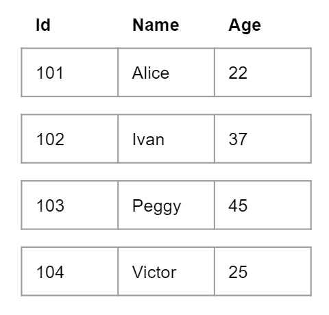
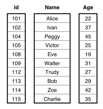
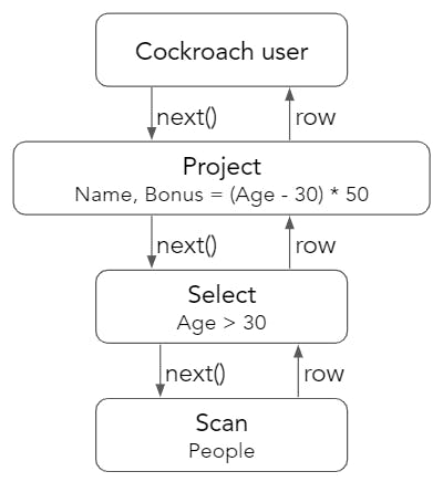
Was that abstract enough for you? We'll get much more concrete next. To illustrate the difference between the Volcano model and the vectorized model, consider a People table with three columns: Id, Name, and Age. In the Volcano model, each data row is processed one at a time by each operator - a row-by-row execution approach. By contrast, in the vectorized execution engine, we pass in a limited-size batch of column-oriented data at a time to be processed. Instead of using a tuple array data structure, we use a set of columns, where each column is an array of a specific data type. In this example, the batch would consist of an array of integers for the Id, an array of bytes for the Name, and an array of integers for the Age. The following pictures show the difference between the data layout in the two models.
Now, let's examine what happens when we execute the SQL query SELECT Name, (Age - 30) * 50 AS Bonus FROM People WHERE Age > 30. In the Volcano model, the top level user requests a row from the Project operator, and this request gets propagated to the bottom layer Scan operator. Scan retrieves a row from the key-value store and passes it up to Select, which checks to see if the row passes the predicate that Age > 30. If the row passes the check, it's returned to the Project operator to compute Bonus = (Age - 30) * 50 as the final output.
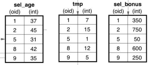
To visualize this, consider a People batch that gets processed by SelectIntGreaterThanInt. This operator would select all Age values that are greater than 30. This new sel_age batch then gets passed to the ProjectSubIntInt operator which performs a simple subtraction to produce the tmp batch. Finally, this tmp batch is passed to the ProjectMultIntInt operator which calculates the final Bonus = (Age - 30) * 50 values.
In order to actually implement one of these vectorized operators, we want to break apart the process into tight for loops over a single column. The following code snippet implements the SelectIntGreaterThanInt operator. The function retrieves a batch from its children, and loops over every element of the column while marking the values that are greater than 30 as selected. The batch along with its selection vector are then returned to the parent operator for further processing.
func (p selGTInt64Int64ConstOp) Next() ColBatch {
    for {
        batch := p.input.Next()

        col := batch.ColVec(p.colIdx).Int64()[:ColBatchSize]
        var idx uint16
        n := batch.Length()
        sel := batch.Selection()

        for i := uint16(0); i < n; i++ {
            var cmp bool
            cmp = col[i] > p.constArg
            if cmp {
                sel[idx] = i
                idx++
            }
        }
    }
}
Note that this code is obviously extremely efficient when you look at it, just based on how simple it is! Look at the for loop: it's not 100% clear without context, but it's iterating over a Go-native slice of int64s, comparing each to another constant int64, and storing the result in another Go-native slice of uint16s. This is just about as simple and fast of a loop as you can program in a language like Go.
The traditional hash joiner
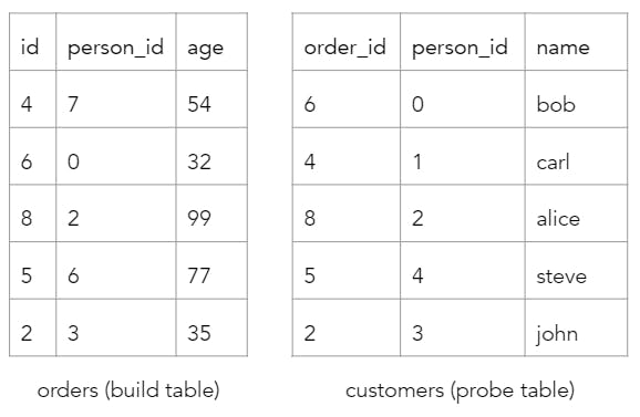
Before we dive into the world of vectorized hash joiners, I wanted to first introduce some hash joiner jargon. Your typical equi-join query probably looks something like SELECT customers.name, orders.age FROM orders JOIN customers ON orders.id = customers.order_id AND orders.person_id = customers.person_id. Upon dissection of this query, we can extract the important information.
A hash joiner is a physical implementation of a relational equi-join operator. Here is a simple algorithm for solving this problem:
Choose the smaller table to be the build table.
Build phase: construct a hash table indexed on the equality key of the build table.
Probe phase: For every probe table row, look up its equality key in the hash table. If the key is found, construct a resulting row using the output columns of the probe table row and its matching build table row.
The vectorized hash joiner
Now that we have a taste of what vectorized execution and hash joiners are, let's take it one step further and combine the two concepts. The challenge is to break down the hash join algorithm into a series of simple loops over a single column, with as few run-time decisions, if statements and jumps as possible. Marcin Zukowski described one such algorithm to implement a many-to-one inner hash join in his paper "Balancing Vectorized Query Execution with Bandwidth-Optimized Storage". This paper laid invaluable groundwork for our vectorized hash join operator.
Many-to-one inner hash join
The algorithm described in Zukowski's paper separates the hash join into two phases; a build phase and a probe phase. The following pseudocode was provided for the build phase.
// Input: build relation with N attributes and K keys
// 1. Compute the bucket number for each tuple, store in bucketV
for (i = 0; i < K; i++)
    hash[i](hashValueV, build.keys[i], n); // type-specific hash() / rehash()
modulo(bucketV, hashValueV, numBuckets, n);
// 2. Prepare hash table organization, compute each tuple position in groupIdV
hashTableInsert(groupIdV, hashTable, bucketV, n)
// 3. Insert all the attributes
for (i = 0; i < N; i++)
    spread[i](hashTable.values[i], groupIdV, build.values[i], n);
Let's try our hand at understanding this part of the algorithm. The ultimate objective of the build phase is to insert every row of the build table into a hash table indexed on its equality key. The hash table we are building is a bucket chaining hash table.
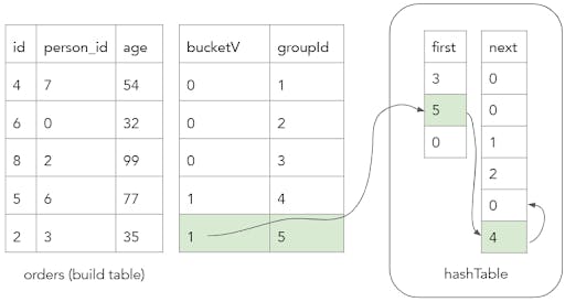
Consider the query SELECT customers.name, orders.age FROM orders JOIN customers ON orders.id = customers.order_id AND orders.person_id = customers.person_id and the following sample tables.
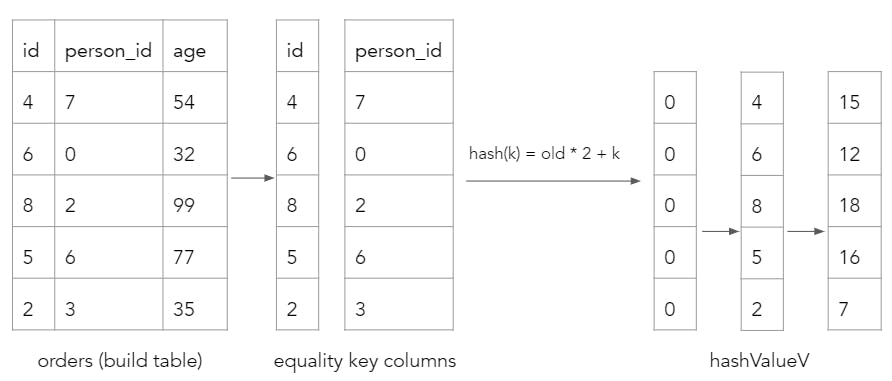
First, we compute the hash value of each build table row by looping over each equality key column and performing a hash. This hash function is unique in that it utilizes the old hash value in its calculation.
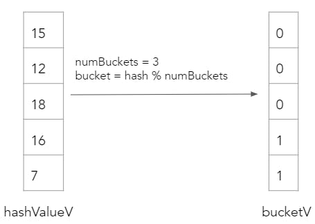
Next, we perform a modulo over the hashValueV array in order to determine the bucket values of each build table row. In this example, our hash table only has 3 buckets.
In the second step, we actually insert the build table rows into the hash table in their corresponding bucketV values. The hashTableInsert function is a simple for loop that inserts each new row to the beginning of the bucket chain in the hash table. It looks like this:
hashTableInsert(groupIdV, hashTable, bucketV, n) {
    for (i = 0; i < n; i++) {
        groupIdV[i] = hashTable.count++;
        hashTable.next[groupIdV[i]] = hashTable.first[bucketV[i]];
        hashTable.first[bucketV[i]] = groupIdV[i];
    }
}
groupIdV is an array that corresponds to the unique row ID of each build table row. The following diagram captures a snapshot of the system state upon insertion of the final row of the build table.
Finally, the last step of the build phase is to perform a spread on every build table output column. This copies and stores all the build table output column values in memory.
Now, that we've stored all the build table rows into a hash table, it's time for the probe phase. The following pseudocode was presented in the paper for the probe phase.
// Input: probe relation with M attributes and K keys, hash-table containing
//     N build attributes
// 1. Compute the bucket number for each probe tuple.
// ... Construct bucketV in the same way as in the build phase ...
// 2. Find the positions in the hash table
// 2a. First, find the first element in the linked list for every tuple,
//      put it in groupIdV, and also initialize toCheckV with the full
//      sequence of input indices (0..n-1).
lookupInitial(groupIdV, toCheckV, bucketV, n);
m = n;
while (m > 0) {
    // 2b. At this stage, toCheckV contains m positions of the input tuples
    //     for which the key comparison needs to be performed. For each tuple
    //     groupIdV contains the currently analyzed offset in the hash table.
    //     We perform a multi-column value check using type-specific
    //     check() / recheck() primitives, producing differsV.
    for (i = 0; i < K; i++)
        check[i](differsV, toCheckV, groupIdV, hashTable.values[i], probe.keys[i], m);
    //  2c. Now, differsV contains 1 for tuples that differ on at least one key,
    //      select these out as these need to be further processed
    m = selectMisses(toCheckV, differV, m);
    // 2d. For the differing tuples, find the next offset in the hash table,
    //     put it in groupIdV
    findNext(toCheckV, hashTable.next, groupIdV, m);
}
// 3. Now, groupIdV for every probe tuple contains the offset of the matching
//    tuple in the hash table. Use it to project attributes from the hash table.
//    (the probe attributes are just propagated)
for (i = 0; i < N; i++)
    gather[i] (result.values[M + i], groupIdV, hashTable.values[i], n);
The objective of the probe phase is to lookup the equality key of every row in the probe table, and if the key is found, construct the resulting output row with the matching rows. To do this, we need to calculate the bucket values of each probe table row, and follow their corresponding bucket chain in the hash table until their is a match or we've reached the end.
However, to do this in a vectorized fashion is a little more complex because we need to break up this process into several, simple loops over a single column. The lookupInitial function computes the bucketV values for each probe table key using the same approach as the build phase. It then populates groupIdV with the first value in the hash table in each bucket. It is also necessary to verify that every row is indeed a match, since different equality keys can reside in the same hash table bucket (due to collision). Thus, we also populate the toCheckV array with the indices (0, …, n). The updated state of the hash joiner is as follows.
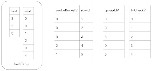
The next part of the probe phase is to verify that the equality key of each probe table row whose index resides in toCheckV is equal to the build table row that the corresponding groupIdV value represents. The toCheckV array is rebuilt with all the probe table row indices that did not match, and the groupIdV values are updated with the next value in the same bucket chain. After one iteration of this process, the state of the hash joiner is as follows.
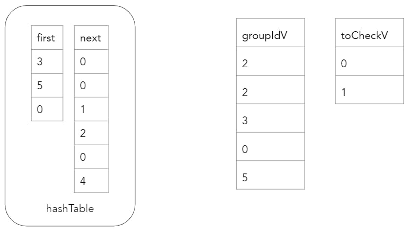
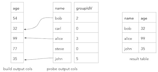
This process can continue until the longest of all bucket chains have been traversed. At the end, the groupIdV array contains the matching build table row ID for each probe table row. If there were no matches, then the groupIdV value would be 0. The final step is to gather together the matching rows by copying the probe table and matching build table output columns column at a time into a resulting batch.
Why did we go through all this trouble?
As we expected, running a series of simple for loops over a single column is extremely fast! The row-at-a-time Volcano model is, by contrast, extremely complex and unfriendly to CPUs, by virtue of the fact that it must essentially behave as a per-row, fully-type-general expression interpreter. Some other major advantages of using vectorized execution include:
Algorithms are CPU cache friendly since we are often operating on sequential memory
Operators only operate on a single data type - this eliminates the need for casting and reduces conditional branching
Late materialization - values are not stitched together until necessary at the end.
Check out the impressive benchmark comparison between Cockroach's pre-existing Volcano model hash joiner and the vectorized hash joiner. The numbers below represent something close to a 40x improvement in throughput. Not bad!
Volcano model hash joiner in CockroachDB today:
BenchmarkHashJoiner/rows=16-8       13.46 MB/s
BenchmarkHashJoiner/rows=256-8      18.69 MB/s
BenchmarkHashJoiner/rows=4096-8     18.97 MB/s
BenchmarkHashJoiner/rows=65536-8    15.30 MB/s
Vectorized hash joiner:
BenchmarkHashJoiner/rows=2048-8     611.55 MB/s
BenchmarkHashJoiner/rows=262144-8   1386.88 MB/s
BenchmarkHashJoiner/rows=4194304-8  680.00 MB/s
I hope you enjoyed learning how our vectorized hash joiner works underneath the hood. Getting to work on such a rewarding project has been an invaluable experience. It gave me the opportunity to really consider things like CPU architecture and compiler optimizations - because at this level, one simple line of code can have non-trivial performance impacts. I'm super grateful for my manager Jordan and Roachmate Alfonso for all their help throughout this internship. Thank you Cockroach Labs, it has been a blast!
P.S.
Cockroach Labs is hiring engineers! If you enjoyed reading about our SQL execution engine, and you think you might be interested in working on a SQL execution engine (or other parts of a cutting edge, distributed database) check out our positions open in New York, Boston, SF, and Seattle.